All published articles of this journal are available on ScienceDirect.

Comparative Analysis of Bilateral Filter and its Variants for Magnetic Resonance Imaging
Abstract
Background:
With the increase in research in the direction of making images noise free a number of algorithms have been designed.
Methods:
The choice of Denoising method will be made in such a way that it reduces or removes noise content on one hand and on the other hand it preserves the information content of the image. Our article focuses on analyzing the performance of bilateral filters and its derivatives for Denoising of MRI images.
Results:
The bilateral filter is a hybridized version of basic range filtering and domain filtering techniques.
Conclusion:
A comparative review of these filters is presented for MRI images taking different altitudes of Gaussian noise added to the image.
1. INTRODUCTION
The idea of a noiseless system is still hypothetical. All the practical systems have some amount of noise present in them. This noise occurs basically due to the design and structure of acquisition devices. The efficiency of various fields of image processing is largely affected by the quantity of noise. Noise is an undesired portion present in the signals which hinders the quality and efficient transmission. While considering Noise in Images, it largely changes the information content present in the Image.
Image denoising is an imperative sub domain in the broad domain of image processing which deals with removing or minimizing the noise levels and reconstructing the information signal [1]. Several techniques have been devised in this direction. While working with medical imaging techniques the presence of noise can largely affect the Physician’s decision in terms of the presence or non-presence of disease. So removal of noise from medical image is an utmost requirement in order to diagnose the disease properly [2]. A lot of research work is being done in the field of denoising of images. An effective denoising model ensures the removal of noise and maintains the quality of image. Noise can affect the feature extraction, selection and classification process in certain applications. In order to remove the noise, two approaches can be used. The first way is related to acquisition of image being done multiple times. The resultant image will be generated by averaging the various versions of captured scene. But this task is a tedious time consuming. The second way removes the noise by applying the post processing methods. Various spatial domain, Frequency domain and wavelet domain filters are proposed in the literature in order to lower down the impact of noise in images [3]. The elimination or removal method for noise can be a linear or a nonlinear method depending upon characteristics of noise [4]. The nonlinear methods outperform the linear methods [5-7]. The removal of noise is not the only task. The most important objective to achieve while designing the system is eliminating the noise and still preserving the valuable information present in the image. With almost every method of denoising a common assumption is made that prior knowledge of type of noise is present. However, this may not be possible with some practical scenarios where the mode and source of acquisition are unknown. Particularly considering Magnetic Resonance Imaging (MRI) the noise can affect the edge points and will degrade the performance of detection systems. Few methods reported in literature which considers automatic calculation of parameters depending upon statistical and mathematical properties of image and noise [8-10]. The image denoising serves to be an important and required step in all image based applications. Various fields of image processing rely upon image denoising algorithms.
 |
(1) |
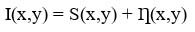
Where I(x,y) denotes the actual input image(corrupted with noise), S(x,y) represents the information content present in the image and Ƞ(x,y) represents noise portion present in an image. The noise affect can either be additive, multiplicative or subtractive depending upon the type of noise and its characteristics defined by is probability density function.
2. TYPES OF NOISE
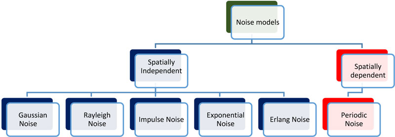
Noise in the image is considered to be a random fluctuation of gray level value resulting in change in brightness and color information in images which are generated by the sensor and circuitry of acquisition devices. All the noise models are mathematically expressed by Probability Density function (PDF). The noise models can be categorized as spatially dependent and spatially independent models. The spatially dependent noise models exhibit the property of a relationship amongst the pixels in spatial sparse form. The gray value from one pixel to the neighboring one varies with certain mathematical relation [11-16]. All the types of noise are discussed briefly as following: (Figs 1 and 2)

2.1. Impulse Noise
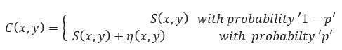
One of the most basic and most widely occurring noises occurring in images due to non-idealities of the image acquisition set is the Impulse Noise. The effect of this noise is generalized as the replacement of few pixels of the noiseless image with new pixels that possess luminance values approximately converging to the minimum or maximum allowed dynamic range [11]. These are short duration noise. It is also known as salt and pepper noise. The efficiency and accuracy of the image based systems depend directly on the amount of noise present in the input image. Eq. (2) describes the characteristics of impulse noise mathematically. Where C(x,y) is the corrupted image due to noise.
 |
(2) |
2.2. Gaussian Noise
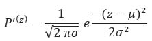
This is additive noise occurring in the images. It is a statistical noise whose PDF matches with Normal distribution curve. In images this noise occurs due to the properties of sensors in the acquisition device.
 |
(3) |
Where symbol z represents gray level, symbol µ represents mean of random variable and σ2 represents variance of z.
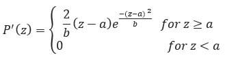
2.3. Rayleigh Noise
This is another type of statistically Independent noise. This is particularly found in Radar range and velocity images. The distribution characteristics are defined by Eq. (4).
 |
(4) |
Where µ represents mean and σ2 represents variance of z.
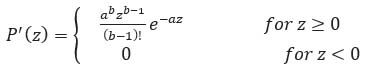
2.4. Erlang Noise
The other name to this noise is Gamma noise. This type of noise generally occurs in laser based systems. The distribution is as given by equation 5 representing the PDF.
 |
(5) |
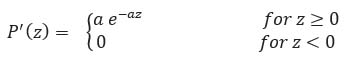
2.5. Exponential Noise
The characteristics of this noise varies exponentially with image gray level values.
 |
(6) |
2.6. Periodic Noise
This noise occurs due to interference of electronic signals generated due to power source for acquisition device. This is generally similar to sinusoidal waveform.
Besides this there is a vast range of objectives to be studied for understanding various kinds of noises. In this article, we attempt to compare four state of the art filters for Image denoising. The noise taken into consideration will particularly be Gaussian Noise and for comparing the efficiency of the filters Magnetic Resonance Image (MRI) is sued. The Gaussian noise is a special case of Rician noise, but considering the practical scenarios in which the amount of noise is high we have preferred Gaussian noise. Magnetic Resonance Imaging (MRI) is a medical imaging technique which provides super detailed image version of human body tissues and organs. MRI has the property of characterization and classification of tissues using their physical and biochemical properties
3. BILATERAL FILTER
Bilateral filter smoothens the image on one hand and on the other hand it preserves the edges by combining nearby pixel values non-linearly [17]. This is a non-iterative filter that is constructed by using a simple logic of similarity of pixels. The closeness or similarity of pixels can be depicted either as closely located in spatial plane or possessing similar gray level values. The operation is carried by using the basic averaging operation implemented in spatial domain. The image is averaged with the weights that decays with the value of dissimilarity amongst the pixels. The value of weights will be decided according to intensity or color value. This filter is hybridization of Range and domain filtering. This hybrid domain filter is very effective at reducing the levels of noise in the image. The pixel value is replaced by the weighted (decided according to similarity of pixels) arithmetic mean of color or intensity values from neighborhood pixels. The weights can be calculated with respect to Gaussian distribution. The weights are generally decided considering both spatial distance and radiometric distances based on Intensity differences.
 |
(7) |
 |
(8) |
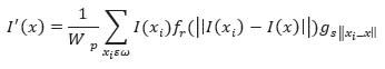
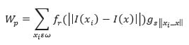
Where Wp are the normalized weights, I’(x) is Bilateral filtered image, x is the current pixel under consideration, ω is the window whose center coincides with current pixel x, fr is the kernel for range filtering, gs is the kernel for domain filtering [18]. The normalised weights make the sum of all weights equal to one. Considering the case where bilateral filter is centred on a brighter pixel, the similarity function takes the value approximately near to one for all those pixels which are on bright side and takes the value approximately equal to zero for all the pixels which belong to dark intensity levels. Then the centre bright pixel takes the updated value as average of all bright pixels located in the vicinity and ignoring all the dark pixels.
The basic bilateral filter can introduce a reverse gradient effect in the image which results in false edges being added to the image. This is the property which makes it somewhere unsuitable for many applications depending upon degradation caused to the edge values. Also this filter adds intensity plateaus which hamper the information content present in the image.
4. ROBUST BILATERAL FILTER
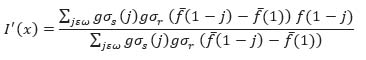
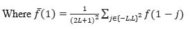
This filter relies upon developing a proxy image which is close to noiseless version of the input image. For this purpose the box filtered version of original image is treated as proxy image [19]. This filter works on generating an estimate of the image known as guide image. It relates and tunes the filter parameters statistically with the input image. The filter operates in iteration mode. It assigns both spatial weights and photometric weight to develop the combined kernel. Robust filter is robust in terms of outliers considering appropriate noise model and convergence method.
 |
(9) |
 |
(10) |
The box filter also introduces smoothing effect and can be controlled by tuning the value of L. Smaller the value of L the optimal results can be obtained. As a small blur can remove the noise, with larger values image content is also blurred.
5. WEIGHTED BILATERAL FILTER
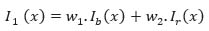
This is a modified version of the robust bilateral filter and utilizes the advantages of both standard bilateral filter and robust bilateral filter. This filter is developed using linear combination of both basic and robust bilateral filter. It combines the estimation in robust to the basic filtering linearly.
 |
(11) |
Where w1, w2 are the filter weights, Ib(x) is the basic bilateral filtered image and Ir(x) is the robust filtered image.
The process works toward optimizing the selection of weights. One way to find optimal value of weights is minimizing mean square error between noiseless image and weighted filtered image. But the noiseless image is never possible in practice. So Stein’s unbiased risk estimate (SURE) is deployed. The optimal weights can be selected by minimizing the value SURE. The MSE can be calculated without the need of noiseless image [19, 20]. By solving the SURE equation which is a quadratic the optimal weights can be obtained. From these calculated weights the final filtered image can be obtained from Eq. (7).
6. METHODS
6.1. Gaussian/Bilateral Filter and its Method Noise Thresholding
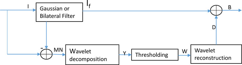
This filter is combination of Gaussian bilateral filter and its method noise Thresholding based on wavelets (GBFMT) [21]. Since all the images contain some amount of noise so the noise removal methods can be evaluated as such and overruling the traditional add and remove method.
In Fig. (3), the architecture for GBFMT is expressed where I represents original input image which may contain noise or may not. IF is the output generated through conventional bilateral filter. The application of Gaussian bilateral filter results in averaging of image and noise while preserving edges and sharp boundaries.
The method noise in this filter comprises noise and all the image details as it is averaged using bilateral Gaussian filtering. So this will contain more sharp edges. The next step will be towards estimating the image details which was removed by Gaussian filtering which can be accomplished by wavelet domain filtering. The true wavelet coefficients will be estimated by information obtained from noisy coefficients. The denoised image will be obtained by summing up the wavelet domain image and the Gaussian bilateral filtered image. This will contain more sharp edges and details as compared to Gaussian bilateral filter. Due to applications of wavelets the noise can be removed from more detailed sub bands which results in higher performance indices. For Thresholding the noise wavelet coefficients Bayes Shrink methodology is deployed. The threshold for particular sub band can be obtained by minimizing Bayesian Risk and is represented by:
 |
(12) |
Where σ2 is noise variance of sub band HH1obtained by median estimation and σw2 is variance value for the wavelet coefficient in the sub band HH1. The estimates can be computed using Bayesian estimation theory [21].
7. RESULTS AND DISCUSSION
To conduct detailed analysis and comparison, the performance of these four filters, MRI data is presented as input to the filter. This comparison can be extended for other types of image but our experimentation clearly focused upon implementation of algorithms on MRI medical images. The experiments are conducted on Intel® core ™ i3-2310 M CPU@2.10Ghz with 4 GB RAM using MTALB 2019b. The evaluation is quantified by calculation of performance metricPeak level Signal to Noise Ratio (PSNR)as defined in Eq. (13).
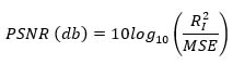 |
(13) |
The input image will be degraded with Gaussian type noise with levels of standard deviation as 10,20,30,40 and 50. Four filters are applied to the images and results obtained. Although MRI images are known to be corrupted with noise but at levels of noise greater than two, the distribution is approximately Gaussian [2]. Therefore to make the algorithm work in practical scenarios, the noise considered in Gaussian in nature.
The type of data for testing purpose are Magnetic Resonance Images. Magnetic Resonance Imaging (MRI) is a medical imaging technique which provides super detailed image version of human body tissues and organs. MRI has the property of characterization and classification of tissues using their physical and biochemical properties. The filters are evaluated by two methods of analysis [21].
(1) Subjective evaluation- This kind of evaluation is done by visual perception. The main focus is towards the data in the image in the form of objects, edges, colors are preserved or not.
(2) Objective evaluation- This kind of evaluation is done in order to check the detailed statistical properties of image. The performance is to be supported by the metrics and then comparative analysis will be done.
7.1. Subjective Evaluation
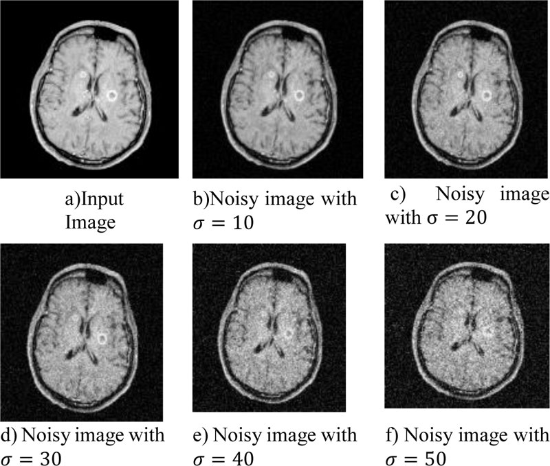
The input MRI image is passed onto four filters with different variance levels of Gaussian noise.
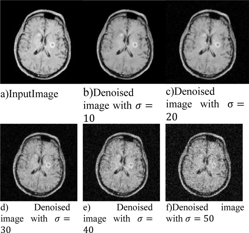
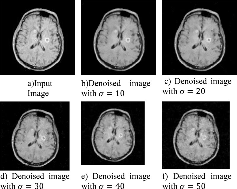
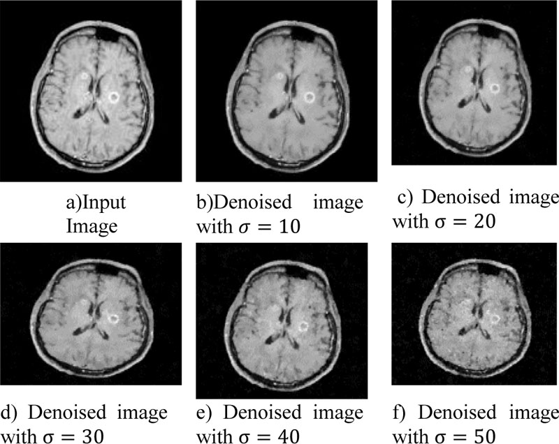
Fig. (4) shows the sample input taken. Fig. (4a) is the original input for testing purpose. Fig. (4b-f) represent the input images with well-known Gaussian noise at 10, 20, 30, 40, 50 standard deviation level. This input will be denoised with the help of four filters as discussed in the previous section namely Bilateral Filter, Robust Bilateral filter, Weighted Bilateral filter, GBFMT. In this section the performance comparison will be made on the base of visual perception of detailing in the input image. The comparative analysis will be done on the basis of edge content preservation, color preservance, shape preservance, etc. The physiologist must be able to use these algorithms and at the very first step a decision is to be made on the visual analysis of the image. Fig. (5) shows the input image and output obtained from standard bilateral filter at 5 different standard deviation levels. Fig. (6) shows the input image and output obtained from robust bilateral filter at 5 different deviation levels. Fig. (7) shows input image and output obtained from weighted bilateral filter at 5 different standard deviation levels. Fig. (8) shows input image and output obtained from GBFMT at 5 different standard deviation levels. The comparative performance alone cannot be judged through visual analysis. As noise may have largely affected and is not removed by the filter and details may not be preserved. The Subjective analysis must be supported by the objective evaluation. For analysis purpose the images can be visually interpreted and the detailing can be cross checked. The performance rating of these filters can be done considering the performance in visual method and finally through the values of PSNR. The combined rating will be able to depict the performance at various levels of Gaussian noise present in MRI images.
| Filters | Different Standard Deviation levels for Gaussian Noise | ||||
| σ = 10 | σ = 20 | σ = 30 | σ = 40 | σ = 50 | |
| SBF | 32.18 | 25.78 | 20.79 | 17.44 | 15.13 |
| RBF | 30.20 | 29.59 | 28.54 | 27.13 | 25.63 |
| WBF | 32.55 | 30.18 | 28.64 | 27.15 | 25.6 |
| GBFMT | 29.56 | 23.58 | 20.10 | 17.69 | 15.87 |
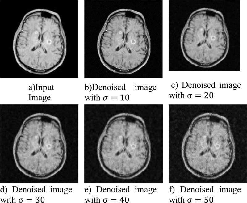
From the visual perception evaluation the performance of both standard and weighted bilateral filter is optimum as the informative details of the image are completely preserved.
7.2. Objective Evaluation
The objective evaluation is done by calculation of parameters like PSNR and a comparative table is presented as shown in Table 1. A number of parameters like Structural similarity, mean square error, and Visual information fidelity are available and proposed in literature but PSNR is one exact crisp parameter that is suitable to determine image quality for a denoising method as PSNR value is inversely proportional to the noise present in the image. The comparison is drawn at 5 different levels and the value of PSNR is calculated.
As shown in Table 1 the values of PSNR fall significantly with increase in the standard deviation values. The images corrupted with known value of Gaussian noise is denoised using filters. From the values obtained as per Table 1 Standard Bilateral Filter and weighted bilateral filter performs the best for Gaussian noise at low standard deviation level but with rising standard deviation levels its performance degrades. For higher standard deviation levels Robust filter is performing optimally. The performance of weighted bilateral filter is best in class as it performs well at both high and low standard deviation levels. The performance of weighted bilateral filter is governed by optimum choice of weights. Therefore the bilateral filters prove to be a suitable choice for Denoising of MRI images as they can perform Denoising at good levels as well as can preserve the details of the image significantly.
The time consumption of SBF,RBF,WBF and GBFMT is calculated and is found to be 1.22 seconds, 1.50 seconds, 1.89 seconds and 2.65 seconds respectively. The time consumption is a measure of algorithm complexity indirectly. Although WBF performs consistently at all noise levels but the time consumption is more. From the timing analysis we can conclude that the time consumption of hybrid domain filter is more as compared to the spatial domain filters. Thus a trade-off need to be made during algorithm selection.
CONCLUSION
This article focuses upon presenting a detailed review of application of bilateral filters for Denoising of images. A number of derivatives of bilateral filter are available in the literature. We have tried to cover the four alternatives which are been extensively used for the Denoising purpose. The performance testing is been done by applying filter on the MRI images and the value of PSNR is evaluated and compared for all four filters. As per our work, the optimum performance for all levels of Gaussian noise is achieved through deployment of Weighted Bilateral filter as it can be tuned appropriately by iterative selection of Weights. This filter satisfies the performance criteria of a Denoising algorithm as it removes the noise and is good at preserving the image details in the form of edges and boundaries.
ETHICS APPROVAL AND CONSENT TO PARTICIPATE
Not applicable.
HUMAN AND ANIMAL RIGHTS
No human or animals were used in this research that are the basis of this study.
CONSENT FOR PUBLICATION
Not applicable.
AVAILABILITY OF DATA AND MATERIALS
Not applicable.
FUNDING
None.
CONFLICT OF INTEREST
The authors declare no conflict of interest, financial or otherwise.
ACKNOWLEDGEMENTS
All authors equally contributed in experimentation, conception and drafting of the article. This work is done in collaboration with Department of E.C.E, UIET, Panjab University Chandigarh Research Lab during 2018-2019.