All published articles of this journal are available on ScienceDirect.

A Review and Experimental Analysis of Denoising Techniques for Medical Images
Abstract
Introduction
Magnetic Resonance Imaging (MRI) and High-Resolution Computed Tomography (HRCT) are crucial for comprehensive diagnosis and treatment planning, as they provide detailed anatomical information. However, noise introduced during image acquisition often degrades the quality of these images, obscuring key anatomical features and complicating accurate diagnoses.
Methods
This study compared the performance of eight denoising algorithms: BM3D, EPLL, FoE, WNNM, Bilateral, Guided, NLM, and DnCNN. Both objective metrics, including Mean Squared Error (MSE), Structural Similarity Index (SSIM), and Peak Signal-to-Noise Ratio (PSNR), as well as perceptual quality metrics, such as NIQE, BRISQUE, and PIQE, were employed to assess their effectiveness.
Results
BM3D consistently outperformed other algorithms at low and moderate noise levels, achieving the highest PSNR and SSIM values while preserving structural integrity and perceptual quality. For high noise levels, conventional algorithms, such as EPLL and WNNM, demonstrated competitive performance in homogeneous areas, preserving fine texture, but were limited by computational complexity.
Discussion
One of the challenges in image denoising is preserving the finer detail structures of images while efficiently removing noise. Finding a balance between the reduction of noise and preservation of image integrity can be a lifesaving challenge, especially in cases where the images are in high detail, such as in the medical world.
Conclusion
This study highlights the trade-offs between denoising quality and computational efficiency among various algorithms for MRI and HRCT images. While BM3D remains a dependable choice for moderate noise levels, advanced deep learning-based methods, such as DnCNN, are better suited for handling significant noise variations without compromising critical diagnostic features.
1. INTRODUCTION
Medical imaging is essential to modern healthcare due to its applications, including detailed profiling in diagnostics, treatment planning, and monitoring of various diseases [1]. The two primary imaging modalities [2] are Magnetic Resonance Imaging [3] and High-Resolution Computed Tomography [4]. Although MRI is functional in revealing detailed information in soft tissues, thus making it unmatched in diagnosing neurological, musculoskeletal, and cardiovascular conditions [5], HRCT [4] is superior in providing detailed anatomical resolution in the lungs, bones, and other structures, and produces high-resolution scans necessary for detecting abnormalities, including lung diseases [6]. However, the images from both MRI and HRCT are often noisy, which degrades image quality and hinders the detection of essential diagnostic information. This is image denoising [7] in medical imaging [8], for which the output should not remove noise, but preserve all important anatomical details [9]. Several factors, including equipment limitations, patient motion, and environmental sources, can cause noise in MRI and HRCT. In medical images, noise is most often categorized as Gaussian noise [10], Rician noise [11], or Poisson noise [12], depending on the imaging modality [13, 14] and the origin of the degradation. Noise can drastically degrade the diagnostic quality of medical images by blurring borders, reducing contrast, and obscuring minute yet crucial information [15]. Clinically, it may lead to misinterpretation, delayed diagnosis, or further imaging to clarify the findings, resulting in higher costs and increased patient exposure to ionizing radiation [16]. Therefore, noise reduction that preserves the integrity of the original structure of MRI and HRCT images is crucial for accurate and efficient diagnosis. Denoising medical images is a challenging problem due to the delicate trade-off required between noise reduction and preservation of essential diagnostic characteristics. Over-smoothing an image to remove noise may lead to the loss of critical anatomical details.
In contrast, under-smoothing will leave the residue of noise, which still degrades the image's utility for diagnosis [17]. A significant problem in MRI and HRCT denoising is that clinically valuable information may be wiped away due to poor contrast. Many pathologies present as subtle contrast changes in the imaging of small tumors or early-stage infections, and over-segmentation in such regions makes it impossible to detect these essential features, potentially leading to their missed detection [18].
Several techniques have been developed to mitigate the noise present in medical images. More conventionally known, these methods are mainly classified into spatial domain and transform domain approaches [19]. In the spatial domain, simple filters such as Gaussian, median, and bilateral filters have been used to smooth images by averaging the intensities of pixels. Simple and computationally efficient, but such filters generally fail to preserve fine details within an image, especially in regions with high-frequency content, such as edges and textures. Techniques, such as wavelet denoising [20], when applied in the transform domain, appear to be more promising. Wavelet transforms decompose the image into different frequency components, allowing high-frequency components, which often contain noise, to be reduced while preserving low-frequency components that contain important anatomical details [20]. It has been helpful in the denoising of HRCT images. Furthermore, crucial information regarding fine lung and bone structures is often contained within their high-frequency content.
There has been considerable attention to the capabilities of advanced algorithms based on machine learning [21] and deep learning [22] for controlling noise in medical images [23]. For example, it has been demonstrated that convolutional neural networks [23] are superior at reducing noise while preserving structural integrity. The latest denoising techniques at the cutting edge include BM3D and DnCNN, which employ different strategies and offer distinct advantages. DnCNN uses deep learning to learn intricate patterns in the noise from training data, whereas BM3D relies on transform-domain processing and collaborative filtering. The clinical scenarios exhibit varying degrees of noise, ranging from optimized conditions with very low noise levels to challenging settings, such as low-dose imaging or rapid acquisitions, which have high noise variance [24]. This variation necessitates the development of denoising algorithms that are robust against various noise levels while preserving the most critical features for diagnosis [25]. In medical image denoising, one of the key challenges is to inhibit noise without compromising over-smoothing and loss of fine structural detail, which are often critical for identifying subtle pathologies, such as early-stage tumors or small lesions.
Denoising algorithms applied to MRI and HRCT images under low and high noise variance conditions are evaluated in this comprehensive study. Using common assessment metrics, such as PSNR, structural similarity index, MSE, and perceptual quality measures like NIQE, BRISQUE, and PIQE, the work quantitatively evaluates the strengths and limitations of such algorithms. Such evaluation should be critical in guiding the selection of appropriate denoising techniques tailored to specific clinical and operational requirements, thereby enhancing the reliability and diagnostic accuracy of medical imaging.
2. LITERATURE REVIEW
Image denoising lies at the centre of interest in image processing, a field that has been a focus of research for several decades, with many methods proposed to remove noise added to high-quality images, primarily through Gaussian noise. Fig. (1a) explains the procedure adopted to find and compile the literature on the review of the medical image denoising. The basis of the first database search is the use of Google Scholar with such keywords: Medical Image Denoising, Gaussian Noise, MRI, HRCT, and Deep Learning. Through this keyword search, 201 articles were retrieved. These were further divided into two major categories, which included the 50 review articles and 151 research articles. Further screening of the research articles identified 36 journal articles and seven conference papers that met the inclusion criterion, and ultimately led to their inclusion in the literature review.
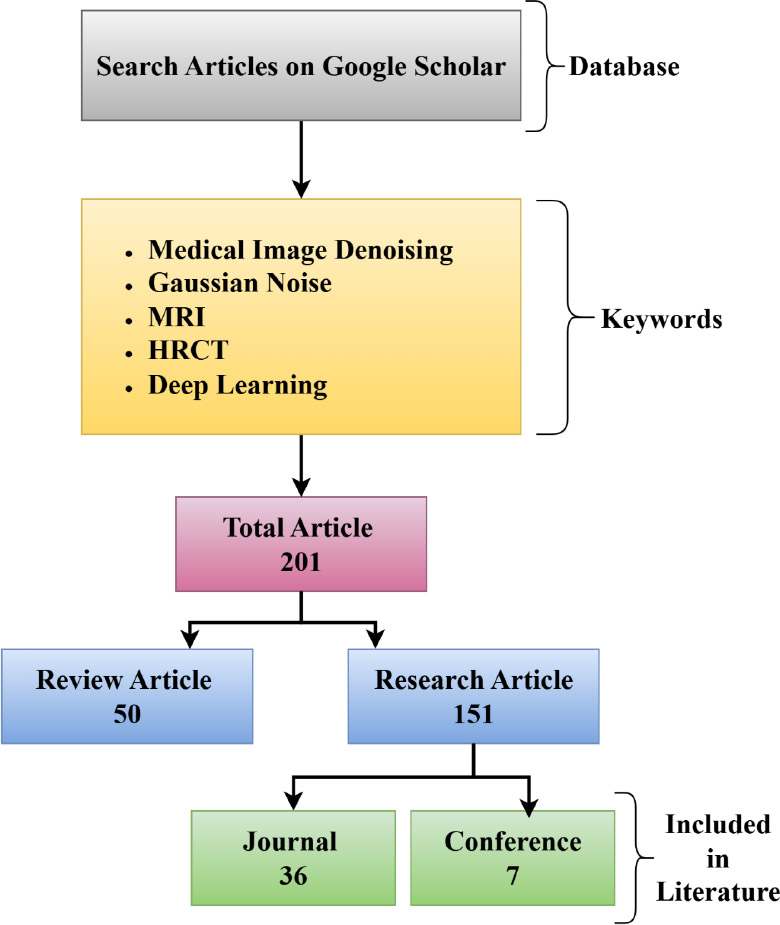
Literature selection workflow for image denoising techniques.
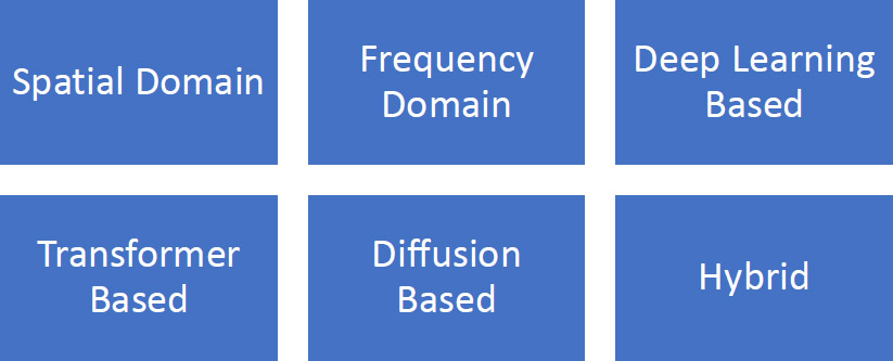
Different categories of image denoising techniques.
This ordered selection ensures a comprehensive and representative overview of both current and past research advancements in the field of medical image denoising. Fig. (1b) shows the different types of image denoising techniques.
2.1. Spatial Domain
The authors have presented an effective technique for removing mixed Gaussian and Random-valued Impulse Noise (RVIN) in a study [26]. The proposed approach consists of two stages: noise categorization and noise reduction. The three-sigma rule, extreme value processing, and the adaptive centre-weighted median filter (ACWMF) form the basis of the noise classifier. In contrast to conventional “detecting then filtering” methods, the noise reduction phase is divided into three steps: preliminary RVIN removal, Gaussian noise removal, and final RVIN removal. First, a noisy image that is roughly distorted by Gaussian noise alone is obtained using RVIN. Then, Gaussian noise is re-estimated, and its denoising is done using BM3D. Finally, the inpainting concept is introduced to further eliminate RVIN. In another study [27], the authors proposed an autoencoder technology for pictures of any size and type, RGB or GS. DVA (Denoising Vanilla Autoencoding) has effectively smoothed Gaussian noise in damaged photos using deep learning techniques. The DnCNN, NAFNET, and Restormer algorithms can remove noise from images; however, a DVA evaluation has been proven to suppress noise to a better extent. In another study [28], the authors proposed a composite multistable stochastic resonance model. The effects of system settings on image noise reduction are discussed, and the dynamic concept of the model in signal identification is presented. An adaptive compound multistable stochastic resonance system is developed to process images and measure radar images under various noise backgrounds, with model parameters optimized using the whale optimization technique. This model addresses the issue of a significant potential barrier and easy saturation in the bistable model. In a study [29], the authors proposed a model for simultaneous super-resolution and blind additive white Gaussian noise (AWGN) denoising by using netdeg and netSR components. The proposed model relies on generating adversarial networks to achieve detailed results while combining both static and dynamic layer features to preserve feature diversity, thereby reducing costs. The model outperforms all the existing methods in the very complex task of concurrent SR and AWGN denoising. The authors of a former study [30] proposed Neighbor2Global, a novel self-supervised framework with noise-level adaptation to remove Poisson-Gaussian noise. Using a GAT-based picture creation strategy, this method solves its training pairs by bringing roughly independent sub-sampled picture pairs from a single noisy image. To efficiently preserve additional texture features, the technique of additional training incorporates an improved reconstruction loss and a regularization term. The experiments demonstrate that our Neighbor2Global performs better than existing techniques in terms of efficiency, particularly for real image photos.
2.2. Frequency Domain
The authors of a study [31] aimed to reduce signal uncertainty by achieving near-optimal sparse representations that utilize both local and non-local correlations of picture content completely and independently. The suggested technique selects different picture data adaptively to exploit both local and non-local correlations. The picture data of interest is retrieved explicitly from clustered rows of patch groups that have comparable image contents, allowing for the exploitation of local correlation. The proposed methodology outperforms previous effective deep learning-based methods in terms of PSNR, SSIM, and visual quality, as indicated by experimental results on picture denoising. One of the efficient techniques used in image denoising, which reduces additive Gaussian noise, is low-rank matrix approximation (LRMA). LRMA performs poorly in the case of eliminating Rician noise from MR images. A novel image denoising method for the case of MR images using the technique of nonlocal low-rank regularization and an extended DoG filter has been proposed in a recent study [32]. The approach enhances patch matching by using a unique nonlocal self-similarity evaluation with a tight frame. An extended DoG filter is applied to the nonlocal low-rank regularization model to eliminate the Rician noise without degrading the edge details. Experimental results are presented to demonstrate that the proposed approach can effectively suppress noise in MR images while preserving more edges and fine details.
2.3. Sparse Models
In a study [33], the authors generalized past learning in image processing and used it for image-denoising processes. It introduces a new prior model named the Group Sparsity Mixture Model (GSMM) for patch group-based past learning, which can represent the sparsity between image patch groups. The paper also introduces a high-efficiency patch group-based image denoising model, which outperforms other models, such as the Field of Experts and the Gaussian Mixture Model. The better version outperformed the state-of-the-art model-based method, WNNM, by running much faster on average. Denoising images is a crucial process in image processing, where classical approaches, such as sparse representation (SR), often incur performance bottlenecks and high computational costs. Deep learning has been found to possess outstanding capabilities for image denoising, and thus, a sparse representation-based network (SRNet) has been developed [34]. The network incorporates a convolutional neural network into the sparse representation scheme, with parameters learned through training. Experimental results indicate that SRNet significantly decreases time cost and enhances denoising performance. In another study [35], the authors proposed a novel multi-scale weighted group sparse coding model (MS-WGSC) for image denoising, utilizing the nonlocal self-similarity (NSS) property of natural images. This model uses multi-scale NSS priors to construct patch groups, and an alternating minimization method is proposed. Extensive experiments demonstrate the model's competitiveness in terms of quantitative metrics, such as PSNR and SSIM, as well as its perceptual quality compared to state-of-the-art methods. In a study [36], the authors introduced a nonlocal self-similar block-based deep image denoising scheme called deep low-rank prior (DLRP). The low-rank property of neighboring NSS patches enables the modeling of a global objective function (GOF) and decomposes it into two subproblems. The deep denoiser is then integrated into the model-based optimization method, which incorporates adaptive noise level estimation, to solve the inverse problem. Stable solutions and flexible and powerful capacity to achieve denoising performance stand out as the leading features of the DLRP method.
2.4. Deep Learning/Self-supervised/GAN-based Models
Deep learning has revolutionized the image denoising problem over the past few years, making it possible to develop models that can directly learn complex spatial priors and noise models from the data. It is possible to learn deep hierarchical representations with deep neural networks automatically, and this significantly increases performance, especially when facing challenging noise conditions, compared to traditional filtering-based techniques [37].
A residual dense neural network (RDUNet) for image denoising has been proposed in a former study [38] based on a densely connected hierarchical network. The model uses convolutional layers, local residual learning, and global residual learning to predict the residual noise of the corrupted image. The algorithm is trained for additive white Gaussian noise and uses a wide range of noise levels. Numerous tests have been conducted using online natural image datasets, and the performance is competitive with that of state-of-the-art networks in the image denoising problem. Additive Gaussian noise levels 10, 30, and 50 are used for comparison. In grayscale images, the gained SSIM values are 0.9297, 0.8193, and 0.7491, while the PSNR values are 34.39 dB, 29.11 dB, and 26.99 dB. The SSIM of the color images is 0.9600, 0.8961, and 0.8465, and the PSNR is 36.68 dB, 31.43 dB, and 29.12 dB. A deconvolution neural network-based image denoising technique is also introduced [39]. A new method to compute loss functions is proposed. The proposed method is tested on the BSD68 and SET12 datasets. Based on the experimental results, the denoising performance of this method is compared to that of the denoising convolutional neural network method. This algorithm's convergence time is reduced by 120% with the same denoising effect. In another study [40], the authors addressed the issue of image denoising when pictures are distorted by non-stationary noise. A deep CNN-based technique for estimating a map of local, patch-wise, standard deviations of noise (referred to as a “sigma-map”) was proposed. The technique demonstrates performance up to 6 dB superior in PSNR to contemporary CNN-based blind image denoising techniques, and up to 0.5 dB superior to other existing methods based on sigma-map estimation, which utilize estimated sigma-maps for image denoising, offering greater flexibility in use. Comparison with an ideal situation shows that the difference in corresponding PSNR values when using ground-truth sigma-map for denoising is under 0.1-0.2 dB and does not exceed 0.6 dB for most noise levels. In another study [41], the authors proposed removing additive white Gaussian noise (AWGN) from images using gradient information, multi-scale features, and feature denoising through a novel deep blind Gaussian denoising network. This network consists of two modules; one generates an intermediate image whose gradient combines the features obtained by the second module to produce the final residual image. The denoising block in the first module helps refine the intermediate image features. By using gradient information from the denoised image and the multi-scale feature block in the second module, the quality of the final denoised image is enhanced. Experimental results show that the new proposed approach surpasses several methods of blind denoising, namely EPLL, BM3D, WNNM, DnCNN, MemNet, BUIFD, Self2Self, and ComplexNet, obtaining up to 2.4dB in PSNR, 0.07 in SSIM, and 0.03 in FOM index compared with the second-best model, in the BSD68, Set5, Set14, SunHays80, and Manga109 image databases. To overcome the disadvantages of the existing image-denoising techniques, the authors of the study [42] demonstrated a CNN model trained on images contaminated with mixed Poisson and Gaussian noise. The resultant trained CNN was provided as an open-source Image plugin that surpasses the traditional fluorescence microscopy denoising methods in SNR improvement and real-time picture denoising within tens of milliseconds. Compared to state-of-the-art fluorescence microscopy denoising approaches, the approach achieves consistently high performance (>8 dB) denoising in less time when evaluated on external datasets.A novel method for structure-preserving noise reduction for FIB-SEM has been devised by the authors [43]. It can leverage the simplicity of Gaussian filtering and locally adjust the filtering to accommodate biological structures. To correct for structural feature fluctuations across the volume before subsequent filtering using a Gaussian function, it employs Optical Flow (OF). The denoising technique outperforms conventional Gaussian filtering, as demonstrated both objectively and qualitatively using datasets from various samples collected under diverse conditions. The authors of the study [44] addressed some of the challenges surrounding wind speed forecasting, including minimizing data noise and selecting optimal model inputs that reveal wind speed variability characteristics. It begins with noise reduction in the wind speed time series using a wavelet soft threshold denoising technique. It determines the ideal model inputs based on the maximum information coefficient calculated by quantifying the correlations between the historical wind-speed data and the predicted targets. A new truncated Gaussian density network based on a convolutional Transformer is created to explain variations in wind speed. After the multi-scale data from convolutional layers are weighted and used to extract temporal information by the Transformer network through self-attention, several linked layers map the outputs to the anticipated objectives. The truncated Gaussian distribution explains the reason for uncertainty in wind speed forecasts; it provides zero probability for negative wind speeds and ensures non-negativity. As a result, the forecasting model develops a loss function based on this. The results for three datasets demonstrate that the suggested method gives reliable probabilistic and accurate deterministic forecasts of wind speed. Hypothesis testing further verifies the efficiency of this approach for both types of forecasting. A two-step denoising technique called GMCM is proposed in another study [45] to address issues, such as high temporal resolution, wide dynamic range, and low power consumption. The two steps consist of motion denoising and Gaussian denoising preprocessing as part of the GMCM method. Adaptive threshold techniques, with a Gaussian temporal distribution, are employed in the first step to determine whether the event streams contain motion-related information. The results demonstrate that Gaussian denoising preprocessing enhances computational performance while also successfully identifying the presence of motion information within the event data stream. On the DVSCLEAN dataset, the GMCM technique achieves SNR scores of 37.22 and 26.79 at 50% and 100% noise ratios, respectively, which represent state-of-the-art performance. The authors of another study [46] proposed a method for unsupervised learning in MRI denoising. First, random noise and content encoders were utilized to separate the noisy artifacts from the content information in low-quality MRI images. Next, the KL divergence loss was utilized for regularization of the noise distribution. Finally, to enhance the realism of the produced denoised images, an adversarial loss was incorporated into the model. To ensure that the content information remains coherent across noisy input and denoised output images, we finally incorporated cycle consistency and perceptual losses. The authors of a previous study [47] built a GAN-based robust denoising network. To extract and learn the features of the input picture, the global residual, which consists of gradient dispersion and feature disappearance, is added to the autoencoder in the generator network. The mean and variance of noise for each generator node are trained and optimized by an optimization algorithm (OA). Its CIFAR-10 dataset exceeds 90% and 99% accuracy in the MNIST dataset. Testing shows that the model's performance in anti-interference has strengthened the defense capabilities of project gradient descent (PGS) and fast gradient sign method (FGSM) attacks by more than a 2% decrease in PSNR and SSIM values. The reliance of brain MRI on CNN disese predictive models for brain tumors and Alzheimer's Disease has also been assessed [48]. The methodology incorporates pre-processing data, stratified k-fold cross-validation, and training four CNN models. The research contrasts the performance of stringent experimentation on four versions of CNN across two brain MRI image datasets, benchmarked by average measures of accuracy, precision, recall, F1 score, and AUC.
2.5. Transformer-based Model
Recently, transformer-based methods have become practical tools for a range of image processing tasks, such as reconstruction, restoration, segmentation, and denoising images [49]. Transformers, initially designed for natural language processing (NLP), have demonstrated significant success in capturing contextual relationships and long-range dependencies, both of which are crucial for comprehending complex visual structures.
In a study [50], the authors have presented a novel Denoise Transformer for real-world image denoising, utilizing Context-aware Denoise Transformer (CADT) units and Secondary Noise Extractor (SNE) blocks. A dual-branch structure can extract both global information and local features, while a hierarchical network learns about the noise distribution. Experiments demonstrate competitive performance, especially in cases of blurred textures and low-light images, without requiring additional knowledge about the noise level or type. The researchers developed TRQ3DNet, a deep neural network that combines a CNN with a transformer for HSI denoising [51]. This includes two branches: one that utilizes 3D quasi-recurrent blocks to extract spatial and spectral correlations, and another that employs Uformer blocks to explore both global and local spatial features. Superior performance has been confirmed by experimental results, which show an improvement of 0.8 in the PSNR value compared to other methods. In a study [52], the authors introduced a heterogeneous window Transformer (HWformer) for denoising images, aiming to strike a balance between distance modeling and denoising time through global window designs that capture global context information while enabling diversified information without prolonging denoising time. HWformer applies a feed-forward network to locally extract information from adjacent patches, shortening denoising time by 30%. Acute Bilirubin Encephalopathy (ABE) is a significant risk factor for neonates, causing disability as well as mortality at a high rate. To tackle this, a Tri-M2MT model is suggested for accurate ABE detection from tri-modality MRI scans [53]. The model incorporates a sophisticated Gaussian Filter, Z-score normalization, a Snake Optimization Algorithm, an Advanced Capsule Network, a multi-transformer technique, and a SoftMax layer for the diagnosis of ABE. The model's performance is evaluated using various metrics, demonstrating improved performance compared to other approaches.
Transformer-based models have shown impressive performance in image denoising, especially in handling Complex noise patterns, High-resolution images, and Global structures and textures often missed by CNNs [54].
2.6. Diffusion Model
The authors have recognized and revisited the diffusion model from a denoising perspective, in a study [55], proposing a new approach called the Diffusion Model for Image Denoising (DMID) that addresses this issue. The DMID technique comprises an adaptive ensemble method that minimizes distortion in the denoised image and an adaptive embedding method that embeds the noisy image within a pre-trained unconditional diffusion model. For both Gaussian and real-world image denoising, the DMID approach provides state-of-the-art performance on distortion-based and perception-based criteria. The authors of the study [56] have proposed a new optimization scheme to remove the combination of Gaussian and impulsive noise from images. The framework is based on a non-convex PDE constraint with two diffusion operators: a fractional order and a local Weickert operator. Although the local and fractional operators preserve the texture and boundaries of the image, the non-convex norm is used to eliminate the impulse component. This section reviews the theoretical characteristics of the proposed PDE-constrained approach, followed by a discussion of some findings on well-posedness in the first subsection. Proximal linearization with a Primal-Dual approach is demonstrated, following the numerical finding of a minimizer in the second part, which includes findings on local convergence. In a study [57], the authors proposed a framework for training single-image Denoising diffusion models, named SinDDM. The architecture employed a multi-scale diffusion process and a lightweight, fully convolutional denoiser to produce high-fidelity samples suitable for tasks, such as style transfer and harmonization, and can be externally supervised. In a study [58], the authors proposed the contextual Conditional Diffusion model (CoCoDiff). This low-dose CT denoising method utilizes a noise estimation network to transform residual images into Gaussian distributions and employs contextual information to mitigate structural distortion. Experimental results demonstrate that the model can recover structural details and generalize well across different noise levels.
2.7. Hybrid Model
In a study [59], the authors combined an anisotropic Gaussian filter (AGF), wavelet transform, and a deep learning-based denoising convolutional neural network (DnCNN) for removing additive Gaussian blur noise (AGBN) from CT scan images. The first step in denoising is to use an anisotropic Gaussian filter and Haar wavelet transforms to remove AGBN from the image. DnCNN is combined with AGF and wavelets for post-processing, which offers the removal of residual noise. AGF was chosen because it is adaptive to edge orientations and hence does not blur in non-uniform noise. PSNR, MSE, and SSIM are used to measure the denoising of images. The average PSNR of the results was 28.28, and the computational time was 0.01666 s. Thus, this reflected that both the original image and the reconstructed version had a small MSE and therefore proved an accurate restoration. The values for SSIM range from 0 to 1.0, where 1.0 represents a perfect match. Values of SSIM close to 1.0 indicate the structural similarity between the denoised CT image and the original. In a study [60], the authors presented a hybrid method for removing noise from digital images using wavelet transform and deep learning techniques. This method decomposes noisy images into their frequency components and then denoises the approximation coefficients using a convolutional neural network, reconstructing the final image. A hybrid model has been shown to utilize wavelet transformations to isolate and reduce noise across varying frequency levels, incorporating a GAN structure to enhance image details [61]. Experiments demonstrate that it outperforms traditional denoising methods in terms of peak signal-to-noise ratio and structural similarity index, making it a suitable tool for practical image denoising applications.
Table 1 summarizes the comparison of different denoising algorithms.
| Category | Key Methods | Advantages | Limitations | Application Domains | Current Trends |
|---|---|---|---|---|---|
| Classical filters | Gaussian, Median, Wiener, Anisotropic Diff. | Simple, fast, low computational cost; no training required | Poor performance on textured/noisy regions; cannot adapt to complex noise patterns | General imaging, real-time systems, and pre-processing steps | Often combined with deep learning (e.g., pre-processing in CNN pipelines) |
| Sparse coding | K-SVD, OMP, Dictionary Learning | Good at preserving edges and textures; interpretable | High computation; requires dictionary training; performance drops with complex noise | Natural images, medical imaging, and hyperspectral data | Less used standalone; now hybridized with deep or self-supervised methods |
| Low-Rank models | Robust PCA, Matrix Completion, NLM variants | Effective in handling structured noise and global patterns | Not suitable for highly textured or local noise; computationally expensive | MRI, CT, video denoising, dynamic imaging | Incorporated in self-supervised frameworks or combined with transform methods |
| Transform-domain methods | Wavelet, Curvelet, BM3D, Shearlet, DCT | Good frequency separation; effective for Gaussian noise; BM3D is state-of-art | May introduce artifacts; fixed transforms may not generalize well; limited adaptivity. | Remote sensing, MRI, visible-infrared fusion | Still baseline for comparisons; used in hybrid and learning-based frameworks |
| Deep learning | CNN, U-Net, ResNet, Transformer | Highly adaptive; learns complex mappings; state-of-the-art performance | Requires large training data; domain shift risk; can hallucinate or remove relevant details | Medical imaging, microscopy, photography, low-dose CT/MRI | Shift toward transformer-based and lightweight models; less reliance on labels |
| Diffusion models | DDPM, Score-based models | High-quality generation; implicit denoising during the reverse process | Very slow inference; not yet mature for real-time medical use | Emerging in high-resolution image restoration, generative tasks | Gaining momentum for unsupervised denoising and inverse problems |
| GAN-based techniques | DnGAN, Pix2Pix, conditional GANs | Sharp outputs; learns perceptual quality; good for blind denoising | Training instability may introduce fake details (hallucination); it is hard to evaluate objectively | CT, low-dose PET, multimodal image translation | Moving toward stabilized variants (e.g., Wasserstein GANs), used in hybrid loss setups. |
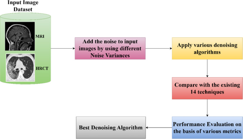
Workflow diagram.
Fig. (2) demonstrates the workflow diagram for evaluating and identifying the best denoising algorithm for multimodal medical images (MRI and HRCT). Firstly, noise has been added to the input images at different noise variances (0.01, 0.05, 0.09, and 0.50), and then various existing denoising algorithms are applied to these images. Then, the performance of the algorithms has been measured on the basis of various evaluation metrics like PSNR, SSIM, etc. Lastly, the best-performing algorithms have been carried out.
3. MATERIAL AND METHODS
3.1. Input Dataset
3.1.1. MR Image
Based on the image characteristics, the present scan is most likely to be identified as a T1-weighted MRI sequence. The T1-weighted image also shows that the gray substance of the brain is darker than the white substance, and the cerebrospinal fluid within the ventricle also appears dark. This sequence is mainly applied to high-resolution anatomical imaging to produce clear boundary demarcation between various structures of the brain and is well employed in the architectural variability of the human brain [62].
3.1.2. HRCT
According to the image characteristics, this scan is probably a High-Resolution Computed Tomography (HRCT) of the chest. In HRCT imaging, lung tissue is imaged in a thin slice thickness of 1-2 mm, which enables excellent depiction of lung structures and minimal parenchymal modifications. Its late phase is preferable for evaluating lung diseases, as it provides excellent resolution and contrast [62].
Fig. (3) demonstrates the dataset images. It shows two images, MRI and HRCT.
3.2. Noise Variance
Noise variance is used to control the strength of noise added to the dataset. The larger the value in the noise variance parameter, the greater the noise that will be spread across the image; otherwise, it would result in very noisy images when using too low a value. One of the most prominent experimental applications of this parameter is noise level simulation, which is used to evaluate the reliability of denoising techniques. Noise is typically added to the medical imaging dataset to simulate real-world conditions. For instance, when working with MRI images, Gaussian noise (or Rician noise) is sometimes introduced to simulate the inherent noise during acquisition. The noise variance may also be measured as an image degradation. The degradation caused by the noise can be calculated by computing the variance of pixel intensity both before and after adding the noise. As noise variance increases, distinguishing between anatomical features and noise becomes more difficult, significantly lowering picture quality [58]. Noise variance is an important consideration when creating or evaluating denoising algorithms for MRI and HRCT. Generally, algorithms are tested against images taken under various levels of noise to ensure that they effectively handle real clinical noise. In this experiment, two datasets, MRI and HRCT, are used, and then different noise variances are applied to these datasets. Four different noise variances are applied to both datasets: 0.01, 0.05, 0.09, and 0.5.
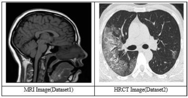
Dataset (MRI & HRCT image) [62].
- 0.01: This is the low-variance noise that indicates that only a small amount of noise is being added to the images. This, therefore, means that the quality of such images is expected to be close to the original, with minimal interference from noise.
- 0.05: This noise variance value is moderate, where the noise in an image becomes easily visible and affects some of the finer details in medical images.
- 0.09: At this value, the noise becomes visible, and the quality of an image starts to degrade; all the important features, such as edges or textures, start to blur or even hide.
- 0.5: This value indicates an extremely high variance in noise, in which noise significantly degrades the quality of the images. Critical anatomical regions in MRI or HRCT scans may become undetectable, making diagnosis and interpretation very challenging.
3.3. Algorithms
3.3.1. Block-matching and 3D Filtering (BM3D)
BM3D is a collaborative filtering method that groups similar image blocks, applies a 3D transform (such as a wavelet or Fourier transform), and then proceeds with denoising in the transform domain. The core idea lies in the similarity of the patches within an image, allowing them to be stacked in a 3D array and collaboratively filtered. BM3D processes the image in two steps that consist of an initial denoising followed by a refinement step [63, 64].
3.3.2. Expected Patch Log Likelihood (EPLL)
This is based on a probabilistic model, where patches from the noisy image are denoised by assuming that they are drawn from a prior distribution. EPLL uses the Gaussian Mixture Model (GMM) as a prior for image patches and tries to find patches that maximize the likelihood given the noisy image. The denoising is performed by solving an optimization problem [65, 66].
3.3.3. Fields of Experts (FoE)
It is based on learning an energy model to capture the statistical properties of the image using filter responses. It uses high-order Markov Random Field (MRF) models, where the denoising task is viewed as an energy minimization problem. The filters used in FoE are learned from data, and the model tries to minimize a loss function that includes both the noisy data and prior knowledge about clean images [67].
3.3.4. Weighted Nuclear Norm Minimization (WNNM)
It works by considering the low-rank properties of image patches. It treats each noisy patch as a matrix and applies nuclear norm minimization to restore the clean patch. It differentiates weights assigned to singular values in the nuclear norm minimization to enhance denoising performance. The approach is successful in exploiting non-local redundancy, especially in images, by relating similar patches [68].
3.3.5. Bilateral Filtering
It is a simple non-linear filter that smooths an image while preserving edges. The idea behind it is the averaging of intensity values among neighboring pixels, taking both spatial closeness and intensity similarity into consideration for this process. This helps in reducing noise while preserving edges [69, 70].
3.3.6. Guided Filtering
It is an edge-preserving filter, albeit more complex than the simple spatial smoothing filters. It employs another guidance image, which might as well be the noisy input image, to compute the filter output. It assumes that the output image should be a linear transform of the guidance image, and based on this assumption, it can maintain sharp edges while smoothing out noise [71].
3.3.7. Non-Local Means (NLM)
It removes noise by replacing the value of each pixel with the weighted average of similar patches from the image. It searches for patches similar to the noisy patch across the entire image, not just within a local neighborhood, and computes the average based on their similarity [72].
3.3.8. Denoising Convolutional Neural Network (DnCNN)
It is a deep learning-based model that uses convolutional neural networks to learn the noise distribution and remove the noise. It shows good performance at both low and high noise levels. It attempts to preserve structural information, which involves maintaining high SSIM scores. It learns automatically from noisy patterns of a complex nature, which requires large datasets for training [73].
3.4. Role of Denoising Algorithms
3.4.1. Feature Preservation
The diagnostic integrity of denoised images in medical imaging is dependent on retaining minor features. Minor yet significant features of an image, termed fine feature details, include subtle textures, edges, and contrast changes. These elements are often crucial markers of pathological disorders. These details are of extreme importance in anomaly detection, such as early-stage cancers, microcalcifications, or small vascular changes on MRI and HRCT scans. Denoising must not suppress the very important characteristics while removing the noise. Minor features usually describe the early signs of disease. In the case of identifying neurological diseases in MRI, the edges of brain structures or microvascular networks are essential. Lung parenchymal texture alterations can be a sign of interstitial lung disorders. During denoising, excessive smoothing can eliminate important gradients and contrasts, leading to misinterpretation of anatomical boundaries. All fine details are retained to ensure accurate size and shape evaluations of small lesions, thereby facilitating early detection and prompt action.
3.4.2. Challenges for Maintaining Fine Features
Aggressive denoising can remove noise, but at the same time drowns high-frequency information containing fine features. It is often challenging to distinguish between noise and real features in medical imaging because noise frequently overlaps or mimics the frequency spectrum of small details. Therefore, algorithms must be sensitive enough to preserve characteristics such as microcalcifications, often drowned by noise. By decomposing images into their frequency components, methods like wavelet-based denoising are effective at selectively removing noise in high-frequency regions while preserving low-frequency components that contain fine details. To keep textures and edges, BM3D uses collaborative filtering and groups patches that are related. This method works very well to remove noise and preserve small details. DnCNN uses large datasets to learn complex noise patterns and separate them from fine details. Due to its ability to maintain fine details easily, it particularly excels at edge information preservation. To preserve edge information, the bilateral filter weights the pixel intensities on the basis of both spatial closeness and intensity similarity. The SSIM, the edge preservation index, and zoomed-in ROI can be used to assess the detail preservation [74, 75].
3.4.3. Homogeneous and Heterogeneous Regions
In medical imaging, regions can be classified as homogeneous or heterogeneous based on the uniformity of their structure, texture, and intensity. The way these regions are treated in image denoising directly affects the clinical interpretation and retention of diagnostic features. In medical images, homogeneous regions are those whose pixel intensities are relatively constant and change little. These regions typically correspond to anatomical structures or tissues that have constant properties, such as solid bone structures, fat, or large regions of healthy soft tissue in MRI images, healthy lung parenchyma, air-filled regions, or solid bone structures in HRCT images. Noise distortion and the risk of over-smoothing are the challenges in denoising homogeneous regions. Heterogeneous regions exhibit noticeable differences in intensity, texture, or structure. They often correspond to diseased regions, such as tumors, lesions, or inflammatory areas, disrupting normal tissue homogeneity, as well as complex anatomical structures, including blood vessels, organ boundaries, or tangled brain networks. Preserving details and avoiding noise overlap make denoising heterogeneous regions challenging. For example, the boundary between gray and white matter in a brain MRI is heterogeneous. The noising must preserve this boundary to ensure that denoising accurately reconstructs anatomy [76, 77].
3.4.4. Small and Large Structure
Medical pictures range from small lesions and fine networks of arteries to gigantic organs and bones, filled with various-sized features. This is what the structures are intended to preserve during denoising: the diagnostic and therapeutic value of the images. Important information about pathological situations can be organized into therapies or tracked as a disease course within small and large structures. Several issues involve noise overlap, blurring, and loss of information with denoising tiny structures. Such large structures in medical imaging involve organs, large bones, or big pathological features like tumors or fractures. These structures appear to act as anatomical markers and often occupy a sizeable portion of the image. Boundary preservation, contrast reduction, edge retention, and global form preservation are some of the challenges in denoising large structures (Table 2) [78, 79].
Table 2.
| Algorithm | Hyperparameter |
|---|---|
| BM3D | • Patch size: 8×8 • Search window: 39×39 • Hard-thresholding followed by Wiener filtering steps as per standard settings. |
| EPLL | • Patch size: 8×8 • Dictionary size: 1024 atoms • K-SVD Thresholding |
| FoE | • Filter size: 3×3, 5×5 • Number of Filters: 8,24 • Patch size: 15×15 |
| WNNM | • Patch size: 6×6, 7×7, 8×8, 9×9 • Search window: 35-60 • No. of Non-Local Similar Patches K =8-14 • Adaptive rank estimation and weighted nuclear norm minimization. |
| Bilateral Filter | • Patch size: 8×8 • Spatial sigma: 3, range sigma: 50, • Kernel size: 5. |
| Guided Filter | • Window Radius(r)= 7 • ε = 0.01 |
| NLM (Non-Local Means) | • Patch size: 7×7 • Search window: 21×21 • h-parameter (filter strength) set empirically based on noise level. |
| DnCNN | • Batch size: 32 • Learning Rate: 1e-4 • Optimizer: ADAM • Activation Function: ReLU |
4. RESULTS AND DISCUSSION
4.1. Performance Metrics
4.1.1. Entropy
Entropy measures the information or randomness in an image [80]. The entropy H of a probability distribution is calculated using the Eq. (1):
 |
(1) |
Where p(i) represents the probability of the i-th outcome, and +n is the total number of outcomes.
4.1.2. Peak Signal-to-noise Ratio (PSNR)
It gives the ratio of the maximum possible power of the signal to the power of noise corrupting it using the Eq. (2) [81].
 |
(2) |
Where MAX is the maximum possible pixel value of the image, and MSE is the Mean Squared Error.
4.1.3. Mean Squared Error (MSE)
It is defined as the average squared difference between the corresponding pixel values of the image and its denoised version as presented in the Eq. (3).
 |
(3) |
Where I(i,j) is the pixel value at position (i,j) in the original image, K(i,j) is the pixel value at position (i,j) in the denoised image, and M and N are the dimensions of the image.
4.1.4. Structural Similarity Index (SSIM)
It measures the structural similarity of two images (Eq. 4) [82].
 |
(4) |
µ1 and µK are the Mean intensities of the original and denoised images,
 and
and
 are the variances of the original and denoised images, σ1K is the covariance between the original and denoised images, and C1 and C2 are the stabilizing constants to avoid division by zero.
4.1.5. Natural Image Quality Evaluator (NIQE)
It is a no-reference metric based on natural scene statistics [83].
 |
(5) |
Where μ, ∑ are the mean and covariance matrix of natural image statistics, µI,∑I are the mean and covariance of the test image's statistics (Eq. 5).
4.1.6. Blind / Referenceless Image Spatial Quality Evaluator (BRISQUE)
It quantifies image quality based on natural scene statistics (Eq. 6) [84].
 |
(6) |
where f(I) is the feature vector of the test image derived from normalized luminance coefficients, and w is the weights obtained during model training.
4.1.7. Perception-based Image Quality Evaluator (PIQE)
It computes image quality by evaluating perceptual distortions (Eq. 7) [85].
 |
(7) |
Where N is the number of image patches, d(i) is the distortion score of the i-th patch based on block-level noise and blur.
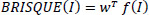
Fig. (4) shows the results at a noise variance of 0.01, where it has been observed that all algorithms produce clear images, except for the Guided algorithm.
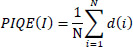
Fig. (5) shows the results at a noise variance of 0.05, where it has been observed that the BM3D, EPLL, and WNNM algorithms produce clearer images compared to other algorithms. NLM and DnCNN also perform well, but not as well as the above-mentioned three algorithms.
The output of different algorithms at a noise variance of 0.01.
The output of different algorithms at a noise variance of 0.05.
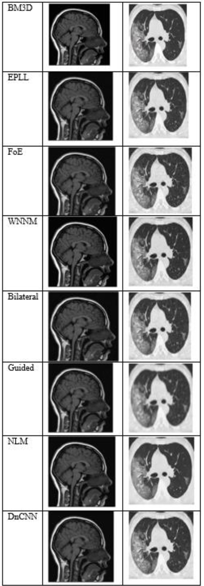
Fig. (6) shows the results at a noise variance of 0.09, where it is observed that the BM3D, EPLL, and WNNM algorithms produce clearer images compared to other algorithms. Another algorithm, DnCNN, also performs well, but not so well as the above-mentioned three algorithms.
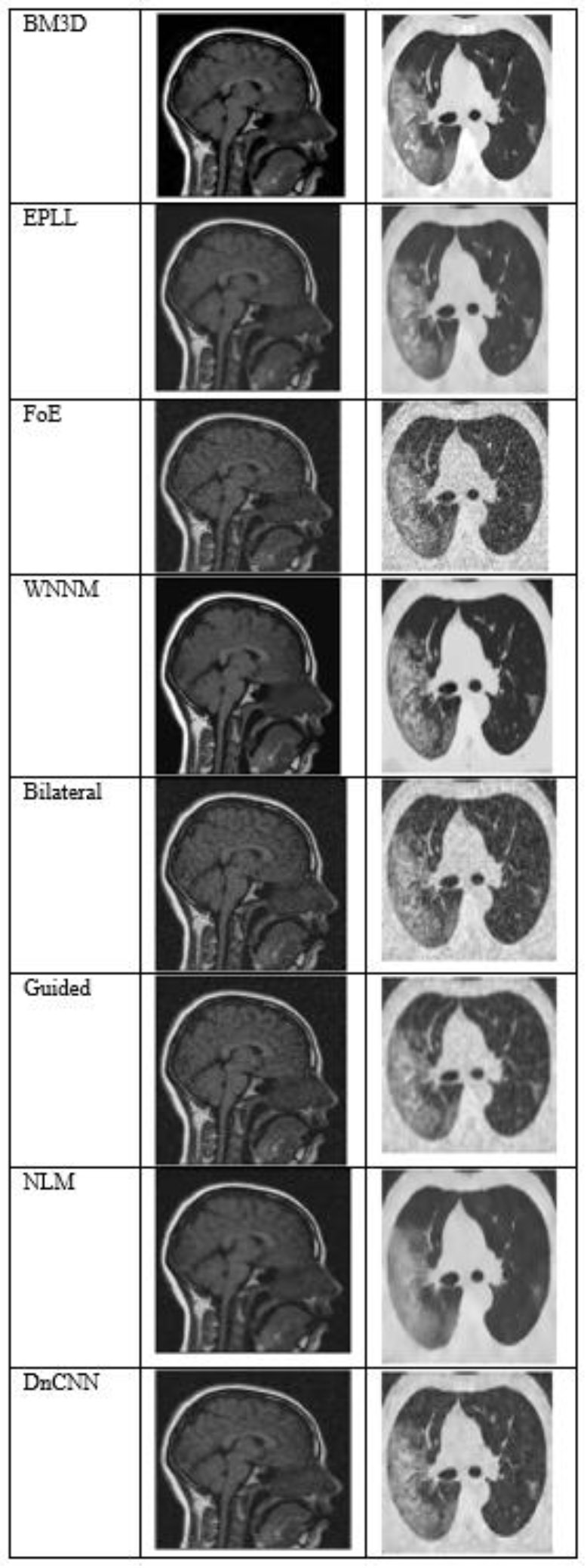
The output of different algorithms at noise variance 0.09.
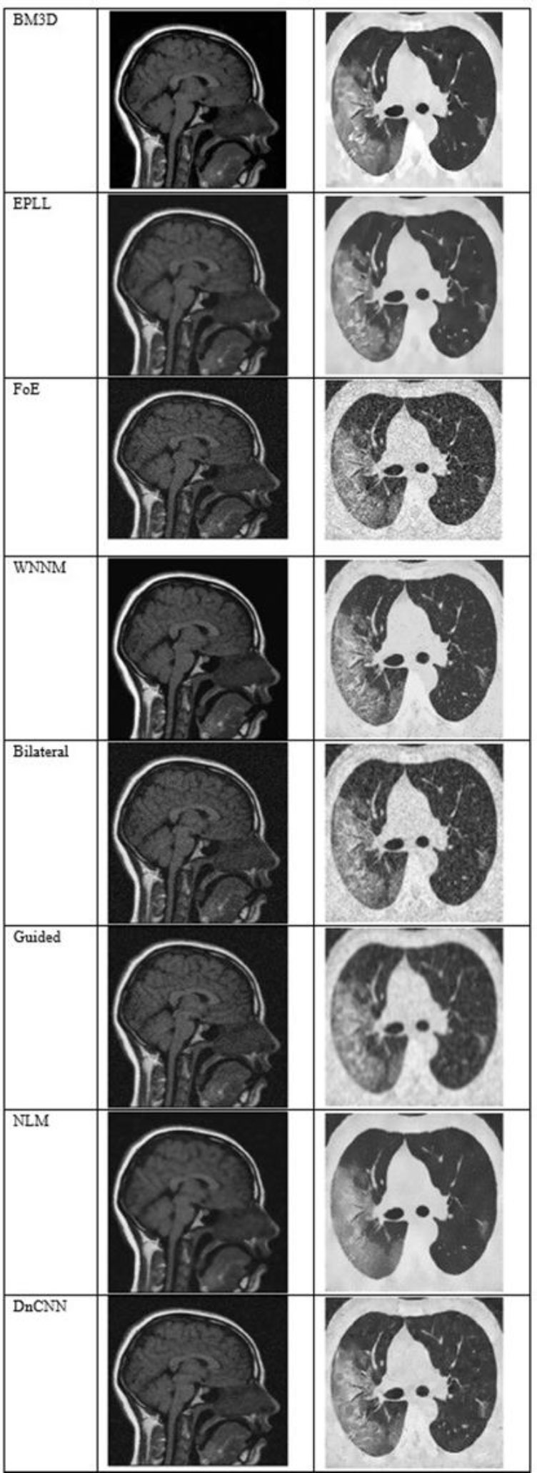
Fig. (7) shows the results at a noise variance of 0.5, where it has been observed that all the algorithms produce blurred images, except for the BM3D algorithm. However, the results of the BM3D algorithm are not so satisfactory. As a result, it has been observed that at a noise variance of 0.5, none of the algorithms performed well.
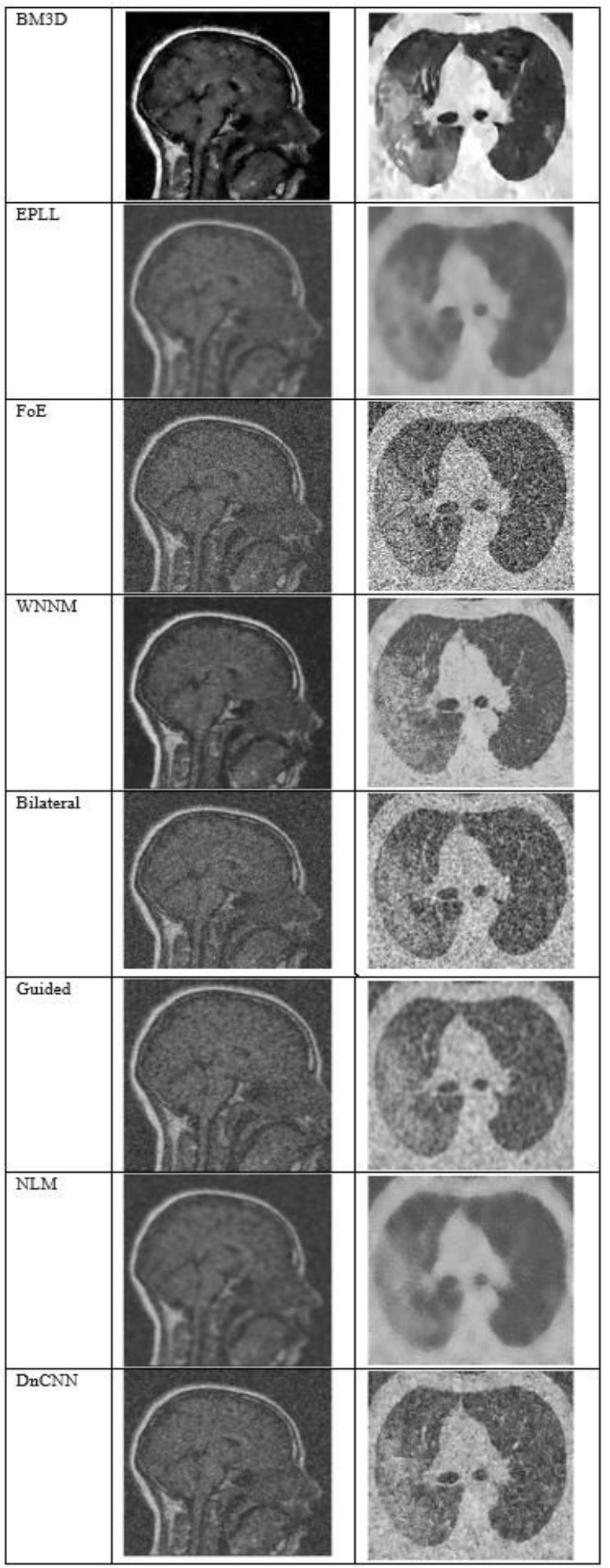
The output of different algorithms at Noise Variance 0.50.
| Algorithms | Noise Variance (NV) | Entropy | PSNR | MSE | SSIM | NIQE | BRISQUE | PIQE |
|---|---|---|---|---|---|---|---|---|
| BM3D | 0.01 | 6.50 | 35.72 | 17.44 | 0.48 | 5.20 | 36.74 | 57.01 |
| 0.05 | 6.53 | 31.10 | 50.45 | 0.36 | 5.59 | 27.53 | 49.32 | |
| 0.09 | 6.53 | 29.38 | 75.04 | 0.31 | 5.74 | 26.98 | 46.77 | |
| 0.50 | 6.57 | 24.18 | 248.50 | 0.18 | 5.97 | 27.52 | 44.78 | |
| EPLL | 0.01 | 6.34 | 32.06 | 52.88 | 0.44 | 7.65 | 23.50 | 50.68 |
| 0.05 | 6.43 | 26.08 | 272.65 | 0.30 | 10.30 | 35.02 | 53.42 | |
| 0.09 | 6.44 | 23.98 | 512.32 | 0.24 | 10.83 | 43.45 | 58.80 | |
| 0.50 | 6.19 | 18.22 | 2642.52 | 0.10 | 33.71 | 43.46 | 70.93 | |
| FoE | 0.01 | 6.99 | 25.28 | 206.06 | 0.21 | 12.78 | 43.01 | 64.14 |
| 0.05 | 7.22 | 16.45 | 1583.62 | 0.07 | 19.88 | 48.43 | 74.74 | |
| 0.09 | 7.24 | 13.85 | 2936.89 | 0.04 | 24.99 | 45.17 | 78.09 | |
| 0.50 | 6.82 | 8.65 | 10548.27 | 0.01 | 69.14 | 43.46 | 85.00 | |
| WNNM | 0.01 | 6.15 | 16.98 | 58.30 | 0.36 | 6.21 | 24.74 | 55.31 |
| 0.05 | 6.29 | 23.25 | 296.70 | 0.22 | 7.00 | 32.91 | 54.90 | |
| 0.09 | 6.06 | 23.06 | 386.19 | 0.25 | 6.96 | 32.16 | 60.30 | |
| 0.50 | 6.44 | 30.16 | 2461.04 | 0.06 | 24.54 | 43.51 | 74.00 | |
| Bilateral | 0.01 | 6.81 | 30.11 | 76.17 | 0.35 | 6.79 | 40.93 | 25.64 |
| 0.05 | 7.00 | 23.91 | 376.38 | 0.21 | 8.74 | 42.60 | 20.67 | |
| 0.09 | 7.06 | 21.83 | 682.93 | 0.16 | 9.10 | 43.19 | 18.74 | |
| 0.50 | 7.17 | 16.60 | 3071.97 | 0.07 | 12.80 | 43.43 | 19.80 | |
| Guided | 0.01 | 6.58 | 29.98 | 78.03 | 0.44 | 7.84 | 49.36 | 56.39 |
| 0.05 | 6.71 | 25.60 | 292.96 | 0.31 | 8.28 | 50.44 | 45.95 | |
| 0.09 | 6.75 | 23.82 | 525.91 | 0.26 | 8.69 | 49.54 | 42.60 | |
| 0.50 | 6.62 | 18.56 | 2566.24 | 0.13 | 9.50 | 44.46 | 34.01 | |
| NLM | 0.01 | 6.33 | 30.64 | 64.61 | 0.33 | 9.77 | 39.14 | 53.71 |
| 0.05 | 6.49 | 24.94 | 284.49 | 0.19 | 10.99 | 43.42 | 62.22 | |
| 0.09 | 6.51 | 23.20 | 495.67 | 0.15 | 12.19 | 43.46 | 65.91 | |
| 0.50 | 6.40 | 18.23 | 2438.70 | 0.07 | 47.04 | 43.46 | 76.40 | |
| DnCNN | 0.01 | 6.46 | 31.27 | 60.75 | 0.39 | 4.15 | 10.18 | 36.57 |
| 0.05 | 6.63 | 25.60 | 285.06 | 0.25 | 4.79 | 19.60 | 37.40 | |
| 0.09 | 6.69 | 23.48 | 538.33 | 0.20 | 5.99 | 20.89 | 39.31 | |
| 0.50 | 6.88 | 17.09 | 2891.19 | 0.06 | 38.74 | 43.49 | 61.55 |
Table 3 presents the performance of several denoising algorithms for dataset 1, where different denoising techniques are applied at varying noise variances. The performance is evaluated using metrics like Entropy, PSNR, MSE, SSIM, NIQE, BRISQUE, and PIQE. BM3D has demonstrated excellent performance at low noise, with a PSNR of 25.45 and a very low MSE of 185.44 at N.V = 0.01. It means that BM3D is capable of removing noise while preserving structural details. However, as the N.V. increases to 0.5, the efficiency of BM3D deteriorates, as the PSNR decreases to 19.02 and the MSE increases to 813.15. The structural similarity, as measured by SSIM, is relatively high at 0.54 but falls to 0.17 under high noise, demonstrating its reduced ability to preserve fine details under noisy conditions. Perceptual quality results from BM3D demonstrate consistent performance, with NIQE values ranging between 5.16 and 6.10 and BRISQUE scores ranging from 13.90 to 10.78. PIQE also demonstrates good perceptual quality retention, with scores ranging from 39.99 to 38.15, which makes BM3D one of the more robust denoising methods. EPLL performs well at low noise levels, reporting a PSNR value of 25.25 and MSE of 195.46 at N.V = 0.01. However, at high noise levels, the performance drops sharply, with PSNR reaching a value of 14.09 and MSE peaking at 2619.92, while N.V = 0.5. Structural preservation is equally affected, as evidenced by a steep decline in SSIM from the value of 0.52 at low noise levels to 0.06 at high noise levels. This reflects a significant loss of structural details, especially at high noise levels. Perceptual quality metrics follow a similar trend, with NIQE growing to 66.36 and PIQE growing to 65.30 at N.V = 0.5, thereby exhibiting a significant degradation in visual quality. FoE fares poorly under all noise levels. Even at low noise (N.V = 0.01), it reports a relatively low PSNR of 23.19 and a high MSE of 312.81. In contrast, at high noise (N.V = 0.5), the PSNR drops to 8.07, and the MSE soars to 10,245.80. SSIM remains consistently low, failing to preserve structural details at all noise levels. The perceived quality is also not very satisfactory for NIQE and BRISQUE, peaking at 80.40 and 85.27, respectively, for N.V = 0.5, which signifies the poorest visual quality in comparison with all testing algorithms. WNNM performs well at low noise with a PSNR value of 22.72, MSE of 187.96, and SSIM of 0.63 at N.V = 0.01. However, its capacity to tolerate higher noise is very low, and at N.V = 0.5, the MSE becomes 2415.21, and the SSIM drops to 0.15. The perceptual quality is also reduced in the presence of high-level noise as NIQE increases to 43.60, BRISQUE to 44.37, and PIQE becomes 73.72. These metrics indicate that WNNM is quite efficient at moderate noise levels but fails to tolerate high noise levels. Bilateral filtering performs reasonably well at low noise, with a PSNR of 23.49 and an MSE of 291.99 at N.V = 0.01. Nevertheless, it was observed to have limited efficacy when the noise levels were substantially higher, as the PSNR value decreased to 14.05 and the MSE increased to 2659.48 at N.V = 0.5. The SSIM reduces from 0.51 to 0.17, indicating that edge and detail preservation decrease with an increase in noise levels. While perceptual metrics like PIQE remain stable (27.71 to 25.04), a high NIQE value (up to 14.30 at N.V = 0.5) indicates visible image degradation under extreme noise levels. Guided filtering does not perform well in terms of structural preservation. SSIM values start at 0.22 at N.V = 0.01 and gradually drop to 0.11 at N.V = 0.5. The PSNR is also relatively low, at 20.51 when N.V is 0.01, and fails to increase significantly with increasing levels of noise. High MSE numbers suggest that it does not significantly reduce noise. Perceptual metrics, such as PIQE scores, improve slightly from 70.60 to 43.25, but still indicate overall poor quality, particularly at higher noise levels. NLM achieves average performance at low noise, with a PSNR of 24.31 and MSE of 241.84 at N.V = 0.01. However, its performance degrades drastically at higher noise levels, where the PSNR falls to 14.41 and the MSE increases to 2429.23 for N.V = 0.5. SSIM is practically negligible at all noise levels, reaching only 0.10 at high noise levels, which signifies a severe loss of structural information. Perceptual metrics, for example, NIQE (60.52 at N.V = 0.5), also indicate significant quality losses. DnCNN exhibits excellent performance at low noise, with a PSNR value of 25.37, an MSE of 189.80, and an SSIM of 0.56 at N.V = 0.01. It is similar to other algorithms; however, its performance degrades at higher noise levels, with the PSNR dropping to 14.26, the MSE rising to 2530.92, and the SSIM reducing to 0.16 at N.V = 0.5. DnCNN exhibits better perceptual quality compared to the rest; it maintains relatively stable values for NIQE, BRISQUE, and PIQE even at high noise levels.
Table 4 presents the performance of several denoising algorithms for dataset 2, where different denoising techniques are applied at varying noise variances. The performance is evaluated using metrics like Entropy, PSNR, MSE, SSIM, NIQE, BRISQUE, and PIQE. BM3D exhibits promising performance even at very low noise levels. It reduces the white noise, achieving a PSNR of 25.45 and an MSE of 185.44 at an N.V. of 0.01, while the SSIM is 0.54, which reveals the structural content of the image. However, it tapers off when the noise levels are higher, as the PSNR decreases to 19.02 and the MSE becomes high at 813.15 at N.V = 0.5. This indicates that BM3D is less effective when the noise is more severe. Structural similarity, as defined by SSIM, reduces dramatically to 0.17, indicating a loss of finer image details under increased noise. Despite this, BM3D achieves relatively good perceptual quality at all noise levels, as confirmed by NIQE scores ranging from 5.16 to 6.10 and BRISQUE scores decreasing from 13.90 to 10.78. The PIQE values varied from 39.99 to 38.15, indicating an essentially constant perceived quality within the considered interval of high noise levels. Under low noise, EPLL also exhibits good performance, with a PSNR of 25.25 and an MSE of 195.46 for N.V = 0.01. However, with increased noise, its effectiveness greatly decreases. At N.V = 0.5, the PSNR decreased to 14.09 while the MSE increased to 2619.92, indicating significant difficulties in noise suppression. Structural preservation also suffers, as the value of SSIM drops sharply from 0.52 at low noise to 0.06 at high noise. This implies that EPLL fails to maintain image details as noise levels increase. Perceptual quality degenerates significantly at higher values of noise since NIQE shoots up to 66.36, and PIQE increases by 65.30. These values show that EPLL cannot afford to retain its acceptable image quality when the noise variance is high. FoE seriously underperforms compared to other algorithms; PSNR values are relatively low, and MSE values are high on all considered noise levels. Even at a low noise level, N.V = 0.01, it achieves only a PSNR of 23.19 with an MSE of 312.81, indicating minimal denoising. More importantly, performance degrades further at higher noise levels (N.V = 0.5), wherein PSNR drops to 8.07 and MSE shoots to 10245.80, thus rendering it the worst of all tested algorithms. SSIM values remain low at all noise level settings, indicating poor structural preservation. The perceptual quality metrics also yield the same results as above, with NIQE and BRISQUE peaking at scores of 80.40 and 85.27, respectively, for N.V = 0.5, indicating that the quality is inferior. WNNM performs well at low noise variance, achieving a PSNR of 22.72, MSE of 187.96, and SSIM of 0.63 at N.V = 0.01. However, its performance degrades as the noise gain increases. At N.V = 0.5, MSE increases to 2415.21, and SSIM decreases to 0.15. It fails to preserve structural details effectively in high-noise conditions. Perceptual quality metrics, such as NIQE and BRISQUE, remain low at high noise levels but degrade severely at higher noise levels. NIQE reaches 43.60 while BRISQUE attains 44.37. PIQE attains 73.72, signifying poor perceived quality when the noise level is high. Bilateral filtering exhibits limited denoising performance at low noise levels, but it is capable of achieving a PSNR of 23.49 and an MSE of 291.99 at N.V = 0.01. Its performance degrades with increases in variance, up to a low PSNR of 14.05 and a high MSE of 2659.48 at N.V = 0.5. The SSIM is at 0.51 for low noise and reduces to 0.17 for high noise, which signifies diminished edge and detail preservation. Perceptual metrics, involving PIQE values, are fairly stable in the range of 27.71 to 25.04, indicating moderate-quality preservation. However, high NIQE values at N.V = 0.5 and 14.30 indicate a visible loss in quality perception. Guided filtering performs poorly in terms of the preservation of structure, as shown in low SSIM scores. At N.V = 0.01, the SSIM is 0.22 and degrades even further to 0.11 at N.V = 0.5. The PSNR is equally low, at only 20.51 at N.V = 0.01, and high MSE values are recorded at all noise levels, indicating that limited noise suppression capability is also achieved. Perceptual quality is not equally well maintained, with PIQE starting at 70.60 and improving modestly to 43.25, suggesting that Guided Filtering does not provide an effective fit for denoising. At low noise variance, NLM offers acceptable denoising performance, reporting a PSNR of 24.31 and an MSE of 241.84 at N.V = 0.01. Beyond this point, the algorithm's effectiveness significantly declines with the rise in variance, and the PSNR value decreases to 14.41, while the MSE reaches 2429.23 at N.V = 0.5. The SSIM is consistently poor, with values of 0.10 at high noise levels, indicating a loss of structural information. The perceptual metrics, such as NIQE and BRISQUE, degrade severely for high noise values, with NIQE attaining a value of 60.52 at N.V = 0.5, indicating significantly degraded perceptual image quality. The DnCNN is also effective at low noise levels, achieving a PSNR of 25.37 dB, an MSE of 189.80, and a SSIM of 0.56 at N.V = 0.01, which is similar to other methods; however, it degrades for higher noise values. At N.V = 0.5, PSNR drops to 14.26, MSE increases to 2530.92, and SSIM falls to 0.16. Although it is dropping, DnCNN still maintains a relatively better perceptual quality than other algorithms, with stable NIQE, BRISQUE, and PIQE values even in scenarios of high noise. Therefore, it demonstrates the great capability of DnCNN in achieving superior visual quality, distinguishing this algorithm as a competitive choice for medical image denoising.
It has been observed that, except for the Guided Filter, which was unable to preserve edge details successfully, most algorithms presented visually clear and good results at low noise levels (variance = 0.01). Techniques such as BM3D, EPLL, and WNNM consistently produced better quality and detail preservation than others in terms of their visual quality and detail preservation at medium noise levels (variance = 0.05 and 0.09). Although their performances were commendable, those of NLM and DnCNN were slightly less accurate and reliable.
| Algorithms | NV (Noise Variance) | Entropy | PSNR (dB) | MSE | SSIM | NIQE | BRISQUE | PIQE |
|---|---|---|---|---|---|---|---|---|
| BM3D | 0.01 | 7.14 | 25.45 | 185.44 | 0.54 | 5.16 | 13.90 | 39.99 |
| 0.05 | 7.13 | 22.67 | 351.77 | 0.32 | 4.13 | 11.87 | 35.70 | |
| 0.09 | 7.21 | 21.80 | 430.02 | 0.28 | 4.84 | 10.37 | 36.10 | |
| 0.50 | 7.56 | 19.02 | 813.15 | 0.17 | 6.10 | 10.78 | 38.15 | |
| EPLL | 0.01 | 7.14 | 25.25 | 195.46 | 0.52 | 4.61 | 1.94 | 30.76 |
| 0.05 | 6.71 | 21.76 | 443.02 | 0.29 | 8.30 | 32.30 | 45.44 | |
| 0.09 | 6.75 | 20.15 | 646.57 | 0.23 | 10.06 | 42.74 | 48.23 | |
| 0.50 | 6.62 | 14.09 | 2619.92 | 0.06 | 66.36 | 43.46 | 65.30 | |
| FoE | 0.01 | 7.70 | 23.19 | 312.81 | 0.60 | 12.66 | 40.60 | 64.15 |
| 0.05 | 7.88 | 15.55 | 1824.00 | 0.29 | 27.19 | 50.08 | 76.32 | |
| 0.09 | 7.78 | 13.11 | 3196.34 | 0.20 | 31.12 | 56.09 | 78.27 | |
| 0.50 | 7.00 | 8.07 | 10245.80 | 0.07 | 80.40 | 43.46 | 85.27 | |
| WNNM | 0.01 | 7.33 | 22.72 | 187.96 | 0.63 | 4.96 | 30.60 | 51.65 |
| 0.05 | 6.99 | 26.76 | 483.53 | 0.38 | 8.42 | 30.91 | 48.58 | |
| 0.09 | 6.49 | 27.34 | 557.23 | 0.28 | 4.74 | 13.56 | 44.13 | |
| 0.50 | 7.19 | 33.69 | 2415.21 | 0.15 | 43.60 | 44.37 | 73.72 | |
| Bilateral | 0.01 | 7.34 | 23.49 | 291.99 | 0.51 | 8.42 | 39.29 | 27.71 |
| 0.05 | 7.51 | 20.96 | 532.50 | 0.39 | 9.65 | 41.28 | 22.64 | |
| 0.09 | 7.58 | 19.31 | 780.48 | 0.33 | 10.07 | 42.83 | 21.62 | |
| 0.50 | 7.52 | 14.05 | 2659.48 | 0.17 | 14.30 | 43.38 | 25.04 | |
| Guided | 0.01 | 7.17 | 20.51 | 579.96 | 0.22 | 7.24 | 48.31 | 70.60 |
| 0.05 | 7.22 | 19.67 | 711.44 | 0.20 | 8.14 | 47.54 | 63.77 | |
| 0.09 | 7.23 | 18.90 | 861.92 | 0.19 | 8.54 | 46.93 | 58.53 | |
| 0.50 | 7.05 | 14.75 | 2273.92 | 0.11 | 8.98 | 45.23 | 43.25 | |
| NLM | 0.01 | 6.97 | 24.31 | 241.84 | 0.45 | 8.24 | 32.55 | 47.41 |
| 0.05 | 6.87 | 21.50 | 471.41 | 0.31 | 10.22 | 42.83 | 62.59 | |
| 0.09 | 6.93 | 19.85 | 691.07 | 0.25 | 19.55 | 43.44 | 66.08 | |
| 0.50 | 6.87 | 14.41 | 2429.23 | 0.10 | 60.52 | 43.46 | 75.69 | |
| DnCNN | 0.01 | 7.19 | 25.37 | 189.80 | 0.56 | 4.05 | 24.16 | 35.86 |
| 0.05 | 7.07 | 22.06 | 416.07 | 0.38 | 6.20 | 23.93 | 39.63 | |
| 0.09 | 7.10 | 20.30 | 627.83 | 0.32 | 7.69 | 27.64 | 38.81 | |
| 0.50 | 7.31 | 14.26 | 2530.92 | 0.16 | 60.90 | 43.78 | 64.93 |
| Algorithm | Processor | Tool Used | Image Size | Image Format | Average Runtime (seconds) |
|---|---|---|---|---|---|
| BM3D | Ryzen 3 | MATLAB | 256 x 256 | .jpg | 1.2 |
| DnCNN | Ryzen 3 | MATLAB | 256 x 256 | .jpg | 2.0 |
| Guided Filter | Ryzen 3 | MATLAB | 256 x 256 | .jpg | 2.3 |
| Bilateral Filter | Ryzen 3 | MATLAB | 256 x 256 | .jpg | 2.7 |
| NLM | Ryzen 3 | MATLAB | 256 x 256 | .jpg | 4.5 |
| WNNM | Ryzen 3 | MATLAB | 256 x 256 | .jpg | 5.0 |
| FoE | Ryzen 3 | MATLAB | 256 x 256 | .jpg | 5.5 |
| EPLL | Ryzen 3 | MATLAB | 256 x 256 | .jpg | 6.0 |
All the algorithms performed poorly at the high-noise level (variance = 0.5), producing significantly distorted and degraded images. At this level of noise, even BM3D, which had demonstrated relative robustness, could not produce outputs appropriate for diagnosis. This result highlights the limitations of current denoising methods in high-noise or low-SNR conditions that are common in low-dose or accelerated medical imaging scenarios.
Table 5 presents a comparison of the execution times for denoising algorithms. A computer equipped with an AMD Ryzen 3 processor and 8 GB of RAM was used to experiment with the execution times of various image denoising algorithms on input images with a pixel size of 256 x 256. With a denoising time of approximately 1.2 seconds, BM3D recorded the fastest execution among all the methods examined. Its moderate computational complexity, owing to block-matching and collaborative filtering approaches, is accountable for its performance. Due to this, BM3D is perfect for real-time processing on mid-range hardware and time-critical applications. The median runtime for the deep learning-based method DnCNN was 2.0 seconds. While it exhibits a low complexity at inference time, it provides a trade-off between speed and denoising quality while running on a CPU, suggesting its feasibility for real-world applications even without GPU acceleration. Only 2.3 seconds were required for the Guided Filter, which was slightly slower than DnCNN and reflected a low to moderate complexity due to its non-linear, intensity–weighted calculations. While it features edge-aware smoothing with a relatively small computational burden, the longer execution time is attributed to the repeated filtering operations that occur during the process. Due to its intensity-based weight and nonlinear nature, which add to the computation, the Bilateral Filter required 2.7 seconds.
Runtimes were larger for more complex methods. In its high-complexity mode, NLM takes 4.5 seconds, as it involves large-scale patch-based comparisons over the entire image, which is a computationally and memory-intensive process. Likewise, the runtimes for WNNM, which uses Singular Value Decomposition (SVD) to estimate low-rank matrices, were 5.0 seconds. With runtimes of 5.5 seconds and 6.0 seconds, respectively, both are considered very high in complexity. Statistical model-based methods, such as EPLL and FoE, were the slowest. Their long processing times are partly caused by EPLL's patch-based inference using iterative Gaussian Mixture Models and FoE's energy minimization approach. Though EPLL and FoE can offer more advanced modeling, their computational demands limit their usage to offline or high-performance computing. BM3D is the most computationally lightweight method. This comparison highlights the trade-offs between runtime performance and denoising accuracy, emphasizing the importance of selecting an algorithm based on the specific operation or clinical requirements.
Fig. (8) illustrates the performance (in terms of running time, measured in seconds) of eight different image denoising algorithms under identical experimental settings. To ensure efficient comparison, every method was evaluated against an image of the same size with the same noise level. The x-axis shows the various denoising algorithms: BM3D, DnCNN, Guided Filter, Bilateral Filter, NLM, WNNM, FoE, and EPLL. The execution time is presented on the y-axis in seconds. BM3D is the most efficient algorithm, with a fast execution time of 1.2 seconds, thereby improving its effectiveness and performance balance. Since it utilizes GPU-accelerated inference and lacks an iterative stage, DnCNN performs well (2.0 s) despite being a deep learning model. The Guided Filter (2.3 s) and Bilateral Filter (2.7 s) have reasonable runtimes. The NLM (4.5 s) and WNNM (5.0 s) are slower because they depend on patch similarity search and matrix operations, respectively. The FoE (5.5 s) and EPLL (6.0 s) are the longest due to their complex optimization structures and statistical prior modeling.
In this study, the evaluation of denoising algorithms was carried out by:
- Visual Analysis.
- Objective Analysis.
- Ablation Study.
4.2. Visual Analysis
Visual analysis of the usual MRI and HRCT images is used to examine the qualitative performance of each denoising algorithm. Special attention was paid to anatomically relevant sites, such as fine pulmonary textures in HRCT and gray-white matter boundaries in T1-weighted brain MRI.
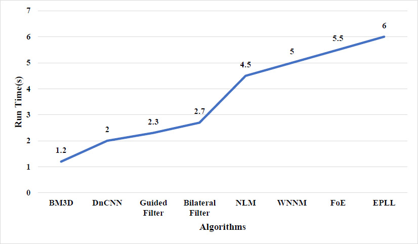
Run-time evaluation of different denoising algorithms.
The visual quality of the denoised images was determined on cropped and zoomed regions of interest (ROIs). The capability of the algorithms to minimize noise while preserving the most essential features, such as tumor borders, ventricular boundaries, or alveolar boundaries, was tested. Such an analysis is crucial, especially in medical imaging, where even slight degradation or excessive smoothing may obscure diagnostic clues. Perceived quality and artifact suppression are illuminated by visual comparisons, and quantitative measurements are corroborated.
4.3. Objective Analysis
An objective analysis of the Structural Similarity Index (SSIM), one of the standard methods for measuring image quality, and the Peak Signal-to-Noise Ratio (PSNR), conducted in conjunction with image inspection, is performed. These metrics numerically analyse the degree of structural faithfulness and noise suppression in comparison with the ground truth. Whereas SSIM determines the similarity between two images based on their structure, contrast, and brightness, PSNR measures the signal-to-noise ratio. To compare performance at low and extreme noise levels, we tested each denoising algorithm with a range of simulated noise levels (e.g., 0.01, 0.05, 0.09, 0.5). These results indicated that in low-noise scenarios, classical methods, such as BM3D, outperformed those based on deep learning, such as DnCNN. However, in moderate and high-noise environments, the latter techniques consistently outperformed the former in terms of both WM and PSNR.
4.4. Ablation Study
We conducted an ablation study, replacing or removing significant parts to understand the role each part plays within the denoising framework. The impacts of batch normalization, residual learning, and depth were investigated in deep learning methods, such as DnCNN. Take, for example, the removal of leftover connections, which led to both slower convergence speed and visible blurring, proving their great importance in maintaining edge acuity. We tested various patch sizes, search windows, and threshold parameters of standard methods, such as BM3D, to investigate how they influenced performance. The ablation findings demonstrated that the balance between noise suppression aggressiveness and the retention of small structural details in medical images is sensitive, and the choices of architecture and parameterization in each technique are justified.
4.5. Limitations of Various Denoising Algorithms
Despite significant advances in medical image denoising, every algorithmic category possesses inherent limitations that affect generalizability and real-world utility. Though computationally fast, traditional filters (e.g., Gaussian, median, bilateral) tend to cause blurring and cannot maintain small anatomical structures, especially in high-noise scenarios. Sparse coding methods are susceptible to parameter tuning and rely on learned dictionaries or patch priors, which may not generalize effectively across different anatomical structures or disease-specific textures. For applications in diverse sites, such as tumors or lesions, the premise of low-rank models' global or non-local redundancy may not be compelling, leading to structural loss or inadequate noise reduction. While transform-domain methods are powerful in identifying multi-scale features, they can result in errors when anatomical structures are not well represented at different scales or when coefficients are over-thresholded. Even with their power, deep-learning-based denoisers often act as “black boxes” with no interpretability, a key issue in clinical decision-making. Their strong performance can be undermined by overfitting some noise models and their typical need for massive annotated datasets, which are often unavailable in specialty domains (e.g., pediatric imaging). Even though diffusion and GAN-based models produce excellent results, they are computationally intensive and can create hallucination features, which is undesirable in a diagnostic environment. Even though self-supervised and cross-modal denoising methods reduce the demand for clean ground truth, they can fail in cases of excessive noise or sparse data. Finally, although promising, multi-tasking and GNN-based frameworks are still in their early stages and often lack standardization, which limits their clinical integration and repeatability.
The denoising methods used have robust performance on benchmark measures and synthetic noise conditions. However, the use of Gaussian noise modeling, a limited dataset, a focus on technical measures without diagnostic evaluation, and untuned generalization across different organs, scanners, or disease states limit the significance and external generalizability of their findings. Extension of these studies into the future will overcome these limitations by incorporating mixed noise models, domain adaptation, and clinical usability evaluation.
4.6. Clinical Limitations
4.6.1. Loss of Diagnostic Detail
Many denoising techniques can inadvertently smooth or obscure fine structural details, such as microcalcifications, vascular boundaries, or subtle tumor margins, resulting in false segmentation or a loss of diagnostic accuracy.
4.7. Clinical Impact After Denoising
To demonstrate the clinical importance of denoising, a comparison is made between noisy and denoised sagittal T1-weighted MRI images. The noisy image may be difficult to diagnose due to its grainy texture and low contrast of tissue structures, as significant structures, such as the brain stem, thalamus, and corpus callosum, are obscured. These make a lot more sense post-denosing, enabling the assessment of subcortical integrity, the inspection of ventricular pathways, and the secure differentiation of gray and white matter. These improvements are not limited to visual interpretation; their direct application to early detection and treatment planning of diseases such as hydrocephalus, multiple sclerosis, and brain tumors firmly places them within the medical field.
To highlight the clinical significance of denoising, a comparison is performed of the visual and anatomical enhancements visible in high-resolution chest CT images. In the initial HRCT model with noise, the clarity of the bronchial walls, pulmonary vessels, and interstitial markings was greatly affected by high-frequency noise, which is important for the identification of certain lung diseases, such as fibrosis, bronchiectasis, or pulmonary infections. Following the denoising process, restored soft tissue contrast and improved visualization of segmental bronchi, vascular branches, and pleural boundaries were observed in the resulting image. Such improvements have a direct impact on the confidence of radiologists, the predictability of lesions, and the probable reduction of false diagnoses. Accordingly, technical validation using PSNR and SSIM was achieved, while the clinical advantage of the denoising procedure was demonstrated by the preservation of diagnostically important structures crucial for accurate thoracic interpretation.
4.8. Clinical Relevance of Image Denoising
It is also crucial to acknowledge the clinical utility of denoising in real-world medical imaging applications. However, our research mainly evaluates denoising algorithms based on technical measures, such as PSNR and SSIM. Noisy images may obscure diseased features or minute anatomical details in medical practice, thereby increasing the likelihood of false discoveries or diagnostic errors. Effective denoising, for instance, is essential for preserving the delicate information of lung parenchyma in low-dose HRCT, where noise levels are amplified to reduce radiation dosage. This enables the detection of pulmonary nodules or early interstitial lung disease [86]. Similarly, denoising increases gray-white contrast in MRI, which is critical for the visibility of small lesions, tumors, or neurodegenerative changes at an early stage. Therefore, image denoising not only enhances aesthetic quality but also improves diagnostic accuracy and radiologist confidence.
4.9. Failure Cases and Performance Degradation Scenarios
Although the evaluated algorithms generally perform well under moderate noise conditions, several failure cases were observed at high noise levels. For example, BM3D performed poorly when applied to images with a high Gaussian noise variance (0.50). In such cases, the patch-matching stage of the algorithm is hindered by the excessive noise, leading to over-smoothing and pronounced artifacts (Fig. 7). The PSNR of dataset 1 decreased by 13.70 dB between noise variances 0.01 and 0.50, while that of dataset 2 decreased by 6.43 dB. Although WNNM performed well in preserving edges, it struggled with homogeneous regions and often introduced patchy textures and low-frequency artifacts when the visual signals in the image were insufficient for low-rank approximation. DnCNN’s performance dropped by nearly 20 dB in PSNR on dataset 1 and by 10 dB on dataset 2, particularly under high noise variance (0.50).
4.10. Data Privacy Concern
To secure the personally identifiable health information (PHI) of patients during collection, storage, processing, and sharing, the clinical and healthcare sectors must implement strict security and governance measures. To block unauthorized access or break-ins, adherence to regulations, such as HIPAA, GDPR, or national health data privacy regulations, is required. This ensures data security through encryption, access control, and audit trails. To ensure the confidentiality of patient data and to further enable the training of the model, the privacy of data regulations in AI-based apps imply that medical data (e.g., removing patient information by removing DICOM header names) should be de-identified or anonymized, and only ethically gathered data with informed consent may be used. It also refers to the threats posed by membership inference or model inversion attacks, which can reveal sensitive personal information. To secure the privacy of data and maintain trust in healthcare AI systems, privacy-preserving techniques, such as federated learning or the use of differential privacy, are required [87].
Safe computing and data privacy have become vital issues in the application of deep learning and image processing techniques in recent years, particularly in the medical sector, regarding the security of patient data. Although the study focuses on denoising methods, the questions related to the processing and location of sensitive imaging data are raised by its implementation in healthcare in the future. To resolve this problem, new frameworks, such as differential privacy and federated learning, offer promising directions. Such methods lessen the likelihood of a breach of privacy by making a central training or inference impossible, as raw medical images are not transferred directly to the server [88].
Another area where decentralized and privacy-preserving recommendation systems hold promise is their application to medical data. The key idea is that user data can be stored locally on a scanner or hospital network to execute denoising models without sending raw data to a third party. Implementing privacy-preserving machine learning is essential for the safe and scalable clinical adoption of denoising frameworks in the future.
Fig. (9) shows comparative denoising results of brain MRI scans processed with eight various denoising methods. A region of interest (ROI) in the brain parenchyma is indicated with a red box in each full sagittal MRI scan image. To assess edge preservation and structural sharpness after denoising, the included zoomed-in patch (inset) enables close inspection of delicate anatomical details, such as ventricles, cortical folds, and grey-white matter interfaces. The zoomed patch is among the cleanest of BM3D, as it has preserved contrast and fine edges. There is a slight blurring of structural edges. EPLL also shows good detail preservation. Compared to BM3D, edges are smoother but still sharp. The noise suppression is well-balanced. WNNM and EPLL show similar results. While relatively smooth with some slight reduction of delicate textures, there is good edge retention. While visually appealing and clear, DnCNN appears too soft in the zoomed area. Texture loss is minimal compared to BM3D and WNNM. Compared to EPLL or WNNM, FoE provides acceptable performance but slightly worse edge detail preservation. NLM's averaging process, under residual noise, is most likely responsible for its minor patchiness and over-smoothing in higher-detail regions. Some edges are maintained through edge-aware smoothness in the Bilateral Filter, but fragile textures are significantly smoothed down. The result appears slightly blurry. In the magnified region, the Guided Filter retains the least level of fine detail. Boundaries are less defined, and textures seem washed out compared to others. BM3D, EPLL, and WNNM achieve the best trade-off between denoising and edge/pixel detail preservation, as indicated by the visual clarity of the zoomed area. In this regard, DnCNN and FoE yield decent results, whereas guided and bilateral filters perform worse.
Fig. (10) contrasts the denoising results of eight different denoising techniques on high-resolution computed tomography (HRCT) lung images. A red rectangle marks a specific region of interest (ROI) within the lung parenchyma in each full HRCT scan image. Venous blood, bronchioles, and soft tissue interfaces are just a few of the small structural features that are retained, as can be appreciated in the inset zoomed-in patch. With excellent edge retention and smooth, sharp textures in the magnified region, BM3D performs outstandingly. There is minimal loss of anatomical detail, as evident in the outstanding clarity of fragile vascular structures. With slight smoothing and carefully preserved textures, EPLL is similarly excellent. In comparison to BM3D, the structure is sharp but possesses slightly reduced contrast. WNNM is a strong rival to BM3D and EPLL because it effectively preserves details while maintaining vessel boundaries with minimal smoothing. While FoE also performs well, it slightly over-smooths the zoomed patch, which makes fine details less crisp. Compared to more traditional methods, such as BM3D or WNNM, DnCNN strikes a good compromise between denoising and texture preservation; however, the image appears slightly oversmoothed. Due to its averaging in patches, NLM exhibits mild blurring in thinner lung structures, which can result in a loss of sharpness in the zoomed-in view. Compared to other methods, bilateral and guided filters have less detail preservation. Particularly in narrow airways and at the borders of arteries, the magnified regions appear mushy, losing sharp edges and contrast.
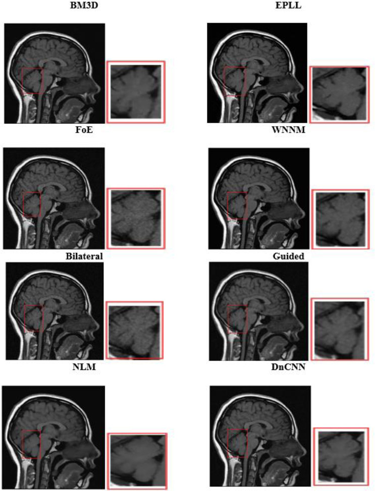
Denoised MRI images with highlighted regions of interest.
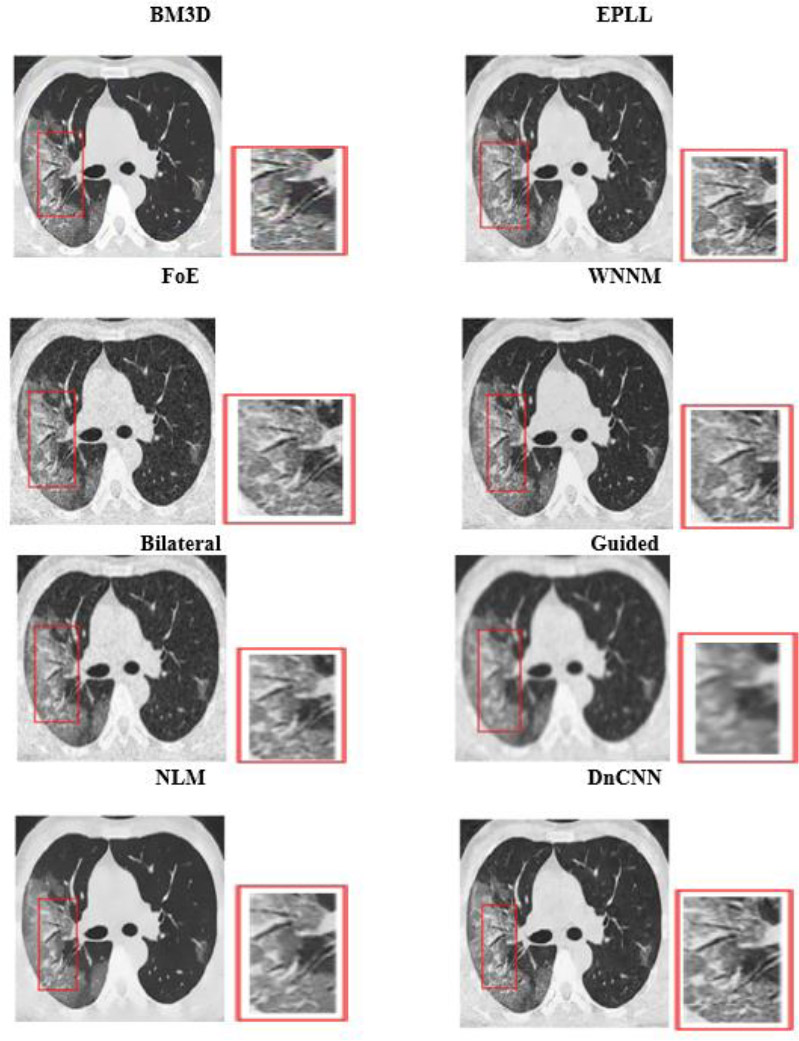
Denoised HRCT images with highlighted regions of interest.
For medical use where the distinctness of small lung structures is critical, BM3D, EPLL, and WNNM have better denoising with anatomical preservation on HRCT images. Though with slight texture loss, DnCNN is competitive.
4.10.1. Algorithm
As seen in Fig. (11), significant anatomical features may be obscured by the extensive smoothing that EPLL applies when denoising images with high noise levels. Fine textures, such as the delicate lines separating different brain regions, become less clear. Subtle features become harder to observe as boundaries and sharp transitions in certain brain areas lose their distinctness. The algorithm’s tendency to remove high-frequency components, often mistaken for noise, can lead to the loss of intricate structures within brain tissue. Although EPLL is an effective noise reduction technique, it suffers from high computational complexity, over-smoothing of important regions, and loss of minute details. These limitations restrict its applicability in clinical imaging, particularly in MRI, where accurate diagnosis depends on preserving fine structural features.
Fig. (12) shows the HRCT image at a noise variance of 0.09 while applying the Bilateral denoising algorithm. Bone outlines become less distinct due to the blurring of the abrupt transitions at the rib, vertebral, and bronchial wall borders. Edge deterioration occurs because the algorithm is unable to distinguish between high-frequency components that are noise-induced and those that are part of actual anatomical structures. As bones and airways become less distinct, it becomes more challenging to identify fractures, calcifications, or blockages in the airways. The image may still appear visually appealing overall, but its clinical utility is limited, as essential diagnostic elements are lost. Although bilateral filtering is effective in reducing noise, it struggles to preserve important edges and can oversmooth delicate anatomical textures, particularly when the noise level is high.
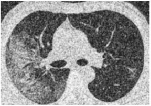
Zoomed MRI image result at noise variance 0.09 with EPLL denoising algorithm.
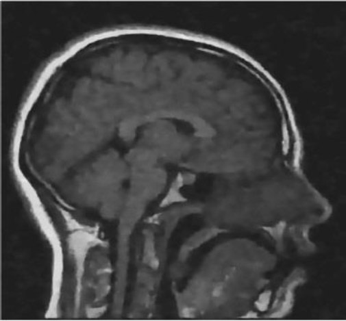
Zoomed HRCT image result at noise variance 0.09 with bilateral denoising algorithm.
CONCLUSION AND FUTURE SCOPE
In this study, the performance of denoising algorithms in MRI and HRCT images is examined under various noise conditions, with a particular focus on how they behave under different noise variations (0.01, 0.05, 0.09, and 0.5). At low to moderate noise levels, BM3D consistently demonstrated good performance, achieving the highest PSNR values and SSIM, while producing images of better perceived quality. Due to its reliability, BM3D is a viable option for environments where anatomy and structure need to be preserved. However, this shows that even at relatively high noise levels (0.5), BM3D fails. Both WNNM and EPLL performed well at low to moderate noise levels; however, they experienced severe difficulties at high noise levels, as indicated by higher MSE and lower SSIM. Although they excel at maintaining uniform areas and delicate textures, their computational complexity makes them challenging to utilize in real-time clinical settings. However, with the help of deep learning's advantages, DnCNN surpassed conventional algorithms in preserving structural and diagnostic qualities at medium noise levels, while showing competitive performance at lower noise levels. Greater variation in noise, however, negatively affected its performance, meaning that additional modifications of the deep learning-based approach are inevitable for high noise levels. FoE and guided filtering performed worse than other methods, particularly in terms of structural integrity and perceptual quality, making them less suitable for medical imaging tasks that require a high level of diagnostic precision. Similarly, NLM, despite its simplicity, could not achieve an optimal trade-off between preserving small and intricate structures and reducing noise. At a noise variance of 0.5, none of the methods were evaluated satisfactorily, highlighting a common challenge in medical imaging: denoising in extremely noisy settings without compromising relevant diagnostic information. BM3D shows competitive results in low to moderate noise levels but underperforms at high noise intensities. To address the limitations observed in high-noise scenarios, this study emphasizes the need for further investigation into advanced denoising techniques, particularly those utilizing hybrid schemes. New techniques, such as explainable AI frameworks, self-supervised denoising, and diffusion models, can potentially enhance both interpretability and performance. Future research incorporating these approaches can lead to denoising systems that are clinically reliable, resilient, and generalizable, ultimately resulting in more accurate and reliable medical diagnoses. Future work can focus on developing context-aware or adaptive algorithms. Future work can also focus on covering mixed and modality-specific noise models (e.g., Poisson, Rician) to evaluate the generality and stability of the method on different imaging conditions.
Additionally, testing on cases of interest for specific organs and diseases will help verify the diagnostic relevance of the denoising performance in real-world applications. Specifically, in the case of medical imaging, unsupervised and self-supervised learning methods have great potential to reduce dependency on pure ground-truth data. Additionally, integrating denoising pipelines with radiomics, quantitative image analysis, and clinical decision support systems can enhance diagnostic accuracy and repeatability. Another emerging trend is the application of privacy-protection measures, like decentralized training architectures and federated learning, to enable collaborative model development without compromising patient confidentiality. Overall, perhaps the most significant barrier—and opportunity—for additional research in medical image denoising is narrowing the gap between algorithmic performance and therapeutic effect.
AUTHORS’ CONTRIBUTIONS
The authors confirm contribution to the paper as follows: A.S.: Writing - Original draft preparation; A.D.: Data analysis or interpretation; B.C.: Data validation; V.K.: Data visualization. All authors read and approved the final version of the manuscript.
LIST OF ABBREVIATIONS
| MRI | = Magnetic Resonance Imaging |
| HRCT | = High-Resolution Computed Tomography |
| BM3D | = Block Matching and 3D Filtering |
| EPLL | = Expected Patch Log Likelihood |
| FoE | = Field of Experts |
| WNNM | = Weighted Nuclear Norm Minimization |
| NLM | = Non-Local Means |
| DnCNN | = Denoising Convolutional Neural Network |
| MSE | = Mean Squared Error |
| SSIM | = Structural Similarity Index |
| PSNR | = Peak Signal-to-Noise Ratio |
| NIQE | = Natural Image Quality Evaluator |
| BRISQUE | = Blind / Referenceless Image Spatial Quality Evaluator |
| PIQE | = Perception-based Image Quality Evaluator |
| RVIN | = Random-Valued Impulse Noise |
| ACWMF | = Adaptive Centre-Weighted Median Filter |
| DVA | = Denoising Vanilla Autoencoding |
| LRMA | = Low-Rank Matrix Approximation |
| GSMM | = Group Sparsity Mixture Model |
| SRNet | = Sparse Representation-Based Network |
| MS-WGSC | = Multi-Scale Weighted Group Sparse Coding Model |
| NSS | = Nonlocal Self-Similarity |
| DLRP | = Deep Low-Rank Prior |
| GOF | = Global Objective Function |
| PGS | = Project Gradient Descent |
| FGSM | = Fast Gradient Sign Method |
| NLP | = Natural Language Processing |
| CADT | = Context-Aware Denoise Transformer |
| SNE | = Secondary Noise Extractor |
| HWformer | = Heterogeneous Window Transformer |
| ABE | = Acute Bilirubin Encephalopathy |
| DMID | = Diffusion Model for Image Denoising |
| CoCoDiff | = Contextual Conditional Diffusion Model |
CONFLICT OF INTEREST
The author Dr. Ayush Dogra is the Editorial Advisory Board member of The Open Neuroimaging Journal.
ACKNOWLEDGEMENTS
Declared none.