All published articles of this journal are available on ScienceDirect.

Patch-Wise Local Principal Component Analysis-based Medical Image Denoising: A Method Noise Approach
Abstract
Introduction
Gaussian noise is often added during the acquisition or transmission of medical images, which can blur important organs and reduce diagnostic accuracy. To address this issue, a hybrid denoising model that combines BayesShrink thresholding in the wavelet domain with Patch-Wise Local Principal Component Analysis (PLPCA) is proposed.
Methods
The framework initially utilises the concept of local patch redundancy by applying PLCA to effectively suppress noise while preserving finer details. The remaining noise is again decomposed using the wavelet transform, with adaptive BayesShrink thresholding applied to refine the coefficients. Subsequently, the reconstructed signal is obtained. The resultant denoised images are then combined to obtain the final enhanced image. HRCTs and MRI datasets were corrupted by Gaussian noise at σ = 10-40 and were validated.
Results
Quantitative analysis based on PSNR, entropy, BRISQUE, NIQE, and PIQE confirmed the consistent high impact of the proposed method across traditional, hybrid, and deep learning baselines. It is worth noting that the approach achieved PSNR values of 31.15 dB at HRCT and 33.00 dB at MRI when σ = 10, as well as at high noise levels (23.95 dB and 22.64 dB, respectively).
Discussion
The proposed method consistently excels over traditional, hybrid, and deep learning-based strategies, as shown by quantitative assessments using PSNR, entropy, BRISQUE, NIQE, and PIQE.
Conclusion
The suggested framework has the strength of suppressing Gaussian noise while retaining anatomical detail. Thus, it is an encouraging option for enhancing the quality of medical image diagnosis in clinical practice.
1. INTRODUCTION
Medical images play a crucial role in modern medicine, as they aid in diagnosis, treatment planning, and disease monitoring. During recording, transmission, or storage processes, these images are often affected by several types of noise, which can degrade image quality and make it harder to interpret them correctly in a clinical environment [1]. Gaussian noise is among the most prevalent forms of noise present in medical imaging systems. It is statistically characterized as a normal distribution of deviations in pixel intensity and is typically caused by thermal noise and electrical fluctuations in the imaging equipment [2]. Gaussian noise has the potential to lower the validity of a diagnosis by blurring significant anatomical features that are crucial in distinguishing diseased from normal structures. Such a noise can adversely impact feature extraction, image segmentation, registration, and finally, the diagnostic process [3]. Image denoising methods, also known as noise reduction methods, are widely used to address this issue. In some cases, conventional denoising methods such as wavelet thresholding, median filtering, and Gaussian filtering have been effective. However, in complex noise environments, the performance of these methods is poor, as they often require trade-offs between noise reduction and edge preservation [4].
Hybrid denoising methods have shown great promise in enhancing diagnostic accuracy and image clarity in the context of medical imaging. Hybrid models can enhance tumor boundaries in brain MRIs and reduce streaking artifacts in CT scans while preserving bone margins. Hybrid models, for instance, can improve tumor boundaries in brain MRIs and reduce streaking artifacts in CT scans while preserving bone margins [5]. Other imaging modalities, such as ultrasound, which can be accompanied by speckle noise, can also be enhanced by these methods. Hybrid methods are highly effective and versatile, as they can be tailored to suit specific anatomical structures and noise characteristics [6].
Researchers have proposed hybrid noise reduction approaches that combine the strengths of multiple denoising algorithms to overcome these limitations. By incorporating edge-preserving filters, statistical or learning-based methods, and spatial-domain and transform-domain techniques, these hybrid models attempt to improve the quality of denoising. High signal fidelity is crucial for clinical decision-making across various radiological modalities, and these advanced methods offer a potential route for enhancing image quality and diagnostic integrity [7].
Gaussian noise poses a significant challenge in medical imaging by degrading image quality and impairing clinical interpretation. Traditional denoising techniques, although useful, often fail to preserve fine anatomical details. Hybrid noise removal techniques offer a promising solution by integrating multiple algorithms to enhance denoising performance, preserve structural integrity, and adapt to complex imaging conditions. As research in this field progresses, these hybrid models are expected to play a critical role in improving the accuracy and reliability of medical image analysis [8].
Medical image denoising is a significant research topic because of the need for high-quality images that reduce noise while preserving fine structural details. Several strategies have been proposed to address this issue. Method-noise convolutional neural networks have been a valuable method for reducing noise in CT images without substantial loss of anatomical features [9]. To enhance edge retention and reduce noise artifacts in CT images, multivariate modelling is applied, which has enhanced accurate diagnostics [10]. Ultrasonic imaging has been effectively applied in hybrid despeckling and total-variation-based filtering methods to improve image clarity and interpretability in clinical analysis [11, 12]. Such studies indicate that deep learning and conventional signal processing methods are undergoing continued development to achieve the reliable denoising performance of various medical imaging modalities.
The remainder of this study is organized in the following manner: Section 2 provides a discussion of relevant literature on existing denoising techniques, including deep learning-based, hybrid, and traditional algorithms. The proposed methodology is discussed at length in Section 3, incorporating BayesShrink thresholding, the wavelet transform architecture, and the PLPCA denoising algorithm. The experimental configuration, dataset description, and performance evaluation metrics are presented in Section 4. Experimental results are presented in Section 5, including qualitative and quantitative comparisons to current state-of-the-art denoising techniques. Section 6 concludes the work with an overview of the findings.
This study has the following key contributions:
(i) To propose a hybrid model of a wavelet BayesShrink and PCA methodology for reducing Gaussian noise in medical images.
(ii) Detailed quantitative and qualitative analysis showing significant improvements over deep learning-based and conventional baselines.
(iii) Highlighting uses in the process of CT and MRI imaging to underline clinical significance.
2. LITERATURE REVIEW
A study [13] proposed a method that employs the Ant Colony Optimization (ACO) algorithm and Two-Dimensional Discrete Cosine Transform (2DDCT) to remove Gaussian noise from medical images. To produce a noiseless reconstructed image as the output, the ACO algorithm identifies the dominant frequency coefficients and eliminates other frequencies that contain significant noise. The proposed method is tested at different standard deviations from both the PSNR and SSIM viewpoints. Satapathy et al. [14] proposed a novel hybridization technique to improve the image quality of noise-degraded images. The proposed decomposition-based method initially splits the image into four quadrants, then high-frequency data is de-noised using conventional denoising techniques. The inverse wavelet transform is applied in order to restore the resulting image. During this process, the wavelet coefficients suppress noisy regions while preserving the image's structural information. For denoising medical images, another study [15] proposed a deep evolutionary network to integrate accelerated genetic methods. Their method achieves improved results on some noisy datasets by adaptively evolving deep structures to maximize noise reduction while preserving image structure.
A denoising method using a biquadratic polynomial model with minimum-error requirements and a low-rank approximation was introduced in a study [16]. The technique had high fidelity in details and efficiently suppressed noise, particularly in images with structured noise patterns. Employing a noise generation network, the researchers [17] introduced a blind medical image denoising method that imitates and removes various types of noise without prior knowledge of the noise distribution. Their method enhances generalization and flexibility in many imaging situations. Atal introduced a deep CNN-based vectorial variation filter for medical image denoising. The architecture uses deep learning and vectorial gradients to improve denoising quality while preserving clinical image contrast and structural information [18]. In another study [19], a novel framework is proposed for filtering images with full control over detail smoothing at a scale level. This iterative, simple, and extendable technique achieves real-time performance and delivers artifact-free segmentation results for a wide range of scale structures, with multiple innovative attributes, surpassing existing edge-preserving filters. A new bitonic filter is constructed, featuring a locally adaptive domain and real-image sensor noise adjustments [20]. The filter enhances noise reduction performance while minimizing processing times. It performs better than block-matching 3D filters for extreme additive white Gaussian noise rates and outperforms other non-learning-based filters on publicly released real noise datasets. The filter's signal-to-noise ratio is 2.4dB worse than that of learning-based methods, but it reduces the performance gap when trained on non-correlated data.
The bilateral and Gaussian filters are linear, local filters that remove details and edges from images without significantly affecting the overall smoothness of the images. The multi-resolution bilateral filter, used on approximation subbands, flattens gray levels and produces a cartoon-like effect. To counteract these problems, a combination of Gaussian/bilateral filters, along with wavelet noise thresholding, is suggested in a study by Rastogi et al [21]. Compared to current denoising algorithms, it performs less well in Gaussian noise conditions but requires less computational time. The non-local means filter is an approach used for denoising noisy images by averaging the weights of pixels. As the noise increases, the filter's performance degrades, resulting in blurring and loss of detail. In another study [22], an integration of the non-local means filter with wavelet noise thresholding has been proposed for enhanced image denoising. The suggested method outperforms wavelet thresholding, bilateral filters, non-local means filters, and multi-resolution bilateral filters in terms of method noise, visual quality, PSNR, and Image Quality Index.
A hybrid model of the Principal Locality Preserving Component Analysis (PLPCA) with the wavelet-domain BayesShrink denoising is used here, unlike the previous hybrid of machine learning and deep learning-based methods [18], which focus primarily on transform-domain filtering or supervised learning using large training sets. This architecture addresses the knowledge gap in how to handle Gaussian noise in medical imaging without requiring extensive training data. In addition, our research addresses two gaps in the literature: the trade-off between noise suppression and fine-detail preservation in denoising methods, and the scalability of these methods to clinical CT and MRI data.
The medical imaging field has recently seen the presentation of several AI-based methods. The Hybrid FrCN (U-Net) method, which combines machine learning with skin cancer segmentation and classification, has demonstrated improved accuracy [23]. An intelligent health model was developed using neural cellular automata to help non-experts interpret medical imaging results, making them more accessible [24]. Additionally, when considering the application of brain MRI analysis, a deep learning-based pipeline that utilised replicator and volumetric networks was created [25]. This pipeline enabled the analysis of complex tumours, comprising feature extraction, segmentation, and survival prediction. Together, these publications emphasize that there has been an increasing role of sophisticated AI architectures in solving complicated imaging problems.
3. MATERIALS AND METHODS
3.1. Dataset Description
Two types of images are used: HRCT and MRI (Fig. 1a-b). The dataset is open source and publicly available [26].
Figure 1a shows chest HRCT in which lung tissue is scanned in narrow slices of 1-2 mm, whereas in Figure 1(b), a T1-weighted MRI sequence is shown.
(a) Dataset1 (HRCT Image), (b) Dataset2 (MR Image)
3.1.1. Preliminaries
3.1.1.1. PLPCA Denoising
A patch-based image denoising technique, referred to as Local Principal Component Analysis (PLPCA), applies the statistical properties of picture patches to denoise images without preserving essential structural information. Small overlapping patches are extracted from the noisy image, passed through Principal Component Analysis (PCA), and the thresholded PCA coefficients are used to eliminate noise components. These patches are then rebuilt and combined into the entire image as part of the denoising procedure [27]. The patches are first vectorised and organised based on their spatial proximity in PLPCA. These clusters are then subjected to PCA, which transforms the data into an uncorrelated space that facilitates simpler separation of signal and noise components. To eliminate components with values less than a certain threshold, typically proportional to the noise level σ, a hard thresholding is applied to the PCA coefficients. To reconstruct the entire denoised image, the denoised patches are initially reconstructed using the inverse PCA transformation and then merged via uniform weighted averaging [28].
- Patch extraction: In this step, the noisy image is divided into overlapping patches for local processing Eq. (1).

Where Pk represents the total no. of patches, and w × w denotes the patch size for local processing.
- PLPCA Denoising: PCA is performed on each local group of similar patches, and thresholding is applied to the PCA coefficients to suppress noise Eq. (2).

Where Xr is the noisy reference patch vector,  r is the mean of all similar patches, U is the PCA basis matrix,. T is the thresholding operator, UT is the projection of the centered patch, Xr is the denoised version of patch X.
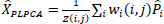
- Aggregation: This step averages the overlapping denoised patches back into a full image Eq. (3).
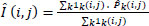
where  is the denoised version of the patch Pk ,
1k is the mask for pixels that are updated by Pk.
is the denoised version of the patch Pk ,
1k is the mask for pixels that are updated by Pk.
3.1.2. Wavelet Transform Decomposition and Reconstruction
One of the powerful tools in analyzing data at multiple scales in image and signal processing is the wavelet transform. It decomposes an image into approximation and detail coefficients, both of which represent high-frequency and low-frequency components, respectively [29]. Due to its computational efficiency and ability to localize features in both the frequency and spatial domains, the Discrete Wavelet Transform (DWT) is widely employed. In a multilevel DWT, an image is decomposed into subbands. The inverse wavelet transform, in combination with processed approximation and detail coefficients, is utilized to reconstruct the original image [30].
3.1.3. Bayes Shrink
One widely used wavelet thresholding method, known as Bayes Shrink, is designed to adaptively denoise each wavelet subband [11]. Through the computation of an adaptive threshold per subband, the fundamental objective is to minimize Bayesian risk (more specifically, mean square error) in the wavelet domain [31, 32]. Soft thresholding is applied by using Eq. (4):

where y is the noisy wavelet coefficient, T is the threshold value, and is the denoised wavelet coefficient after thresholding.
Then, the BayesShrink threshold is designed to minimize MSE Eq. (5):
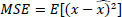
Where x is a true wavelet coefficient, is the estimated wavelet coefficient, and E is the expectation operator.
3.2. Proposed Methodology
|
Step 1: Add Gaussian Noise to the input image Eq. (6). | |
 |
(6) |
 |
(7) |
 |
(8) |
 |
(9) |
 |
(10) |
 |
(11) |
 |
(12) |
Proposed methodology for image denoising.
Figure 2 demonstrates a hybrid image denoising system that successfully removes Gaussian noise, preserving fine details in medical images through the integration of wavelet-based BayesShrink thresholding with Patch-Wise Local Principal Component Analysis (PLPCA). To simulate real-world degradation during recording or transmission, a noisy image is generated by adding Gaussian noise to a clean input image at various standard deviation levels (σ = 10, 20, 30, 40). The PLPCA algorithm is then used to initiate the denoising process. To achieve this, the noisy image is segmented into overlapping local patches, which are then grouped based on their spatial similarity. A mean-centered matrix is formed for each group of related patches. After transforming this matrix into a decorrelated space by Singular Value Decomposition (SVD), noise-dominated components are eliminated with a thresholding operation. A denoised image is formed by combining and reconstructing the patches.
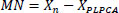
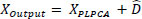
After the PLPCA stage, the PLPCA-denoised image is then subtracted from the noisy original image to find a residual or method noise. This residual contains any remaining noise and the fine picture details that were omitted in the first denoising process. To further enhance denoising, the technique decomposes noise into frequency subbands via a wavelet transform, using filters designed to isolate high-frequency detail components from low-frequency approximation components.
The coefficients are then adaptively thresholded using the BayesShrink method, which minimizes Mean Squared Error (MSE) in each subband based on the local statistical properties of the signal and noise. After thresholding, a denoised version of the residual image is obtained by reconstructing the wavelet coefficients via the inverse wavelet transform. The resulting output image is subsequently achieved by adding this reconstructed image to the PLPCA-denoised image pixel-wise. This process produces a high-quality image with reduced noise and diagnostic features preserved by blending the detail-enhancement ability of wavelet-based thresholding with the structural-preservation ability of PLPCA. This method is especially suited to medical imaging, where accurate interpretation and analysis rely on retaining anatomical structure while reducing noise.
4. EXPERIMENTAL RESULTS AND DISCUSSION
Using the MATLAB platform, all of the experiments were conducted on a PC with an AMD Ryzen 3-3250 U processor running at 2.6 GHz and 4 GB of RAM. To perform the experiment, two types of images, MRI and HRCT, are used [26]. For research purposes, it is a publicly accessible collection of medical images. These dataset images get infected by Gaussian noise at different noise standard values σ=10,20,30,40. In this section, the performance of the proposed method is evaluated using two forms of analysis: subjective and objective. Both methods provide complementary insights into the performance and quality of the denoising algorithm. Human viewers view denoised images visually during subjective testing. The main concerns of this qualitative testing are whether the denoised image appears visually realistic, whether small features and structural edges are preserved, and whether artifacts, such as blurring, ringing, or over-smoothing, are apparent. During the research, denoised results from several approaches were compared graphically across several levels of noise. The proposed algorithm generated diagnostically useful, high-quality images, retaining important anatomical and textural details while minimizing visual noise.
Quantitative assessments of denoising quality are made available through objective metrics. A variety of standard metrics are used for assessing image quality, including PSNR, entropy, BRISQUE, NIQE, and PIQE. PSNR measures the fidelity of the denoised image compared with the ground truth. Improved performance is reflected in a higher PSNR. Entropy is an information retention measure that balances between detail preservation and noise suppression. The No-reference perceptual quality estimators BRISQUE, NIQE, and PIQE assess distortion without reference to ground truth. Compared to experimental results, the proposed technique outperformed most existing traditional and learning-based schemes, particularly in high-noise scenarios, with comparable or improved PSNR values and outstanding perceptual quality scores at different noise levels.
4.1. Entropy
It measures the randomness and the amount of information in an image Eq. (13) [33].
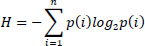
Where pi is the probability of the ith intensity level, and summation is over all gray levels in the image.
4.2. PSNR
PSNR stands for Peak Signal-to-Noise Ratio. It measures the difference between the original and denoised image Eq. (14) [34].
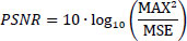
Where Max is the maximum possible pixel value of the image, and MSE is the mean squared error.
4.3. Blind / Referenceless Image Spatial Quality Evaluator (BRISQUE)
It quantifies image quality based on natural scene statistics Eq. (15) [35].

where f (I) is the feature vector of the test image derived from normalized luminance coefficients, and w is the weights obtained during model training.
4.4. Natural Image Quality Evaluator (NIQE)
It is a no-reference metric based on natural scene statistics Eq. (16) [36].
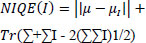
where µ, Σ are the mean and covariance matrix of natural image statistics, µI, ΣI are the mean and covariance of the test image’s statistics.
4.5. Perception-based Image Quality Evaluator (PIQE)
It computes image quality by evaluating perceptual distortions Eq. (17) [37].
Where N is the number of image patches, d(i) is the distortion score of the i-th patch based on block-level noise and blur.
Table 1 presents the performance evaluation of various denoising algorithms based on the Entropy, PSNR, BRISQUE, PIQE, and NIQE metrics for Dataset 1 images with rising Gaussian noise levels (σ = 10, 20, 30, and 40). A combination of these metrics assesses perceptual quality, structural content retention, and image fidelity. The trend in performance of learning-based, hybrid, and conventional methods is well illustrated by the data. At all levels of noise, the proposed method consistently outperforms the others. With 31.15 dB at σ = 10 and 23.95 dB at σ = 40, it achieves the highest PSNR. This demonstrates its resistance to increasing noise. Additionally, the proposed method achieves competitive entropy scores (around 4.0), indicating effective information retention. Among all σ values, it also yields the lowest BRISQUE, NIQE, and PIQE scores, which implies outstanding perceptual quality and minimal distortion from the observer's perspective. Interestingly, for σ = 40, PIQE scores drop to 21.25, which shows that the method effectively removes noise without compromising visual clarity. The poor noise-suppression ability of traditional filters, like Median, Gaussian, and Bitonic, is evident from their low PSNR value (typically 5.6-6.0 dB) and greater BRISQUE and NIQE values. Though some of the above methods have higher entropy, this is not due to preserved detail but due to preserved noise. Rolling Guidance and DWT perform reasonably well in terms of entropy and PSNR, but degrade as noise increases, especially in perceptual metrics such as PIQE, where scores exceed 60. At low levels of noise, learning-based methods such as BF-CNN, NGRNet, and ODVV perform relatively well. ODVV performs the best among them, maintaining good scores at larger σ and achieving a PSNR of 27.45 dB at σ = 10. However, their BRISQUE/NIQE values are not always optimal, and their performance is compromised with increasing levels of noise. While they perform better than the proposed approach, other hybrid methods, such as GA, GBFMT, and NLFMT, yield better PSNR than traditional filters. For instance, at σ = 10 (28.39 dB), GBFMT achieves a respectable PSNR; however, its perceptual measures are weaker. What is surprising is that NLFMT involves a trade-off between fidelity and visual quality, as indicated by its higher BRISQUE and PIQE scores, despite its robust PSNR performance. The proposed method offers a near-perfect trade-off between perceptual and quantitative denoising performance, making it well-suited for medical image improvement tasks where distortion should be kept to a minimum while anatomical information is preserved. It is a significant improvement over existing classical, learning-based, and hybrid methods by virtue of its insensitivity to noise levels as well as its consistently low distortion rates.
| Method | σ | Entropy | PSNR | BRISQUE | NIQE | PIQE |
|---|---|---|---|---|---|---|
| DWT | 10 | 3.99 | 21.61 | 48.46 | 6.82 | 62.80 |
| 20 | 3.81 | 20.45 | 47.19 | 6.43 | 63.67 | |
| 30 | 3.78 | 20.33 | 46.14 | 6.51 | 66.02 | |
| 40 | 3.87 | 13.32 | 47.78 | 6.54 | 64.65 | |
| GA | 10 | 4.34 | 23.44 | 44.65 | 7.18 | 51.00 |
| 20 | 4.15 | 21.24 | 40.19 | 6.12 | 55.22 | |
| 30 | 4.47 | 20.68 | 43.99 | 5.94 | 61.21 | |
| 40 | 4.07 | 14.38 | 43.47 | 6.35 | 63.91 | |
| BF-CNN | 10 | 5.941 | 23.53 | 44.75 | 6.17 | 56.62 |
| 20 | 5.469 | 21.54 | 44.51 | 5.97 | 57.77 | |
| 30 | 5.521 | 18.59 | 45.39 | 4.58 | 51.80 | |
| 40 | 5.093 | 17.22 | 43.45 | 5.74 | 52.85 | |
| NGRNet | 10 | 6.33 | 25.72 | 30.60 | 4.96 | 35.65 |
| 20 | 6.99 | 22.76 | 30.91 | 5.42 | 38.58 | |
| 30 | 6.49 | 23.34 | 33.56 | 4.74 | 44.13 | |
| 40 | 6.19 | 19.69 | 36.37 | 4.60 | 33.72 | |
| ODVV | 10 | 7.01 | 27.45 | 25.90 | 4.16 | 29.99 |
| 20 | 7.00 | 23.67 | 25.87 | 4.13 | 27.70 | |
| 30 | 6.95 | 21.80 | 26.37 | 4.84 | 26.10 | |
| 40 | 6.56 | 20.02 | 30.78 | 5.10 | 28.15 | |
| GBFMT | 10 | 3.21 | 28.39 | 45.88 | 4.61 | 32.06 |
| 20 | 3.28 | 22.55 | 45.33 | 4.22 | 25.87 | |
| 30 | 3.30 | 19.31 | 44.67 | 4.10 | 24.81 | |
| 40 | 3.30 | 17.11 | 44.47 | 4.00 | 24.62 | |
| NLFMT | 10 | 3.25 | 28.38 | 47.83 | 6.09 | 45.99 |
| 20 | 3.30 | 22.54 | 46.50 | 4.62 | 32.51 | |
| 30 | 3.27 | 19.31 | 45.55 | 3.81 | 29.54 | |
| 40 | 3.25 | 17.12 | 46.16 | 4.47 | 30.75 | |
| Rolling Guidance | 10 | 6.79 | 14.65 | 31.10 | 5.68 | 44.73 |
| 20 | 6.91 | 14.30 | 42.45 | 14.14 | 62.92 | |
| 30 | 6.92 | 13.86 | 46.72 | 16.73 | 68.21 | |
| 40 | 6.93 | 13.41 | 48.55 | 24.48 | 69.31 | |
| Bitonic | 10 | 7.24 | 5.67 | 38.57 | 5.78 | 25.62 |
| 20 | 7.18 | 5.69 | 37.02 | 6.52 | 36.87 | |
| 30 | 7.29 | 5.93 | 40.89 | 5.79 | 26.98 | |
| 40 | 7.29 | 5.98 | 40.89 | 5.79 | 26.98 | |
| Gaussian | 10 | 7.26 | 5.76 | 36.79 | 7.45 | 54.36 |
| 20 | 7.22 | 5.77 | 39.33 | 8.01 | 61.14 | |
| 30 | 7.28 | 6.04 | 38.68 | 7.16 | 47.99 | |
| 40 | 7.28 | 6.09 | 38.68 | 7.16 | 47.99 | |
| Median | 10 | 7.34 | 5.60 | 42.34 | 7.94 | 14.60 |
| 20 | 7.23 | 5.67 | 42.84 | 7.59 | 19.21 | |
| 30 | 7.44 | 5.77 | 41.64 | 8.35 | 13.55 | |
| 40 | 7.44 | 5.82 | 41.64 | 8.35 | 13.55 | |
| GBFMT | 10 | 3.21 | 28.39 | 45.88 | 4.61 | 32.06 |
| 20 | 3.28 | 22.55 | 45.33 | 4.22 | 25.87 | |
| 30 | 3.30 | 19.31 | 44.67 | 4.10 | 24.81 | |
| 40 | 3.30 | 17.11 | 44.47 | 4.00 | 24.62 | |
| NLFMT | 10 | 3.25 | 28.38 | 47.83 | 6.09 | 45.99 |
| 20 | 3.30 | 22.54 | 46.50 | 4.62 | 32.51 | |
| 30 | 3.27 | 19.31 | 45.55 | 3.81 | 29.54 | |
| 40 | 3.25 | 17.12 | 46.16 | 4.47 | 30.75 | |
| Proposed | 10 | 3.91 | 31.15 | 26.38 | 5.46 | 24.23 |
| 20 | 3.95 | 27.30 | 27.28 | 4.08 | 24.11 | |
| 30 | 3.98 | 25.29 | 27.01 | 4.44 | 21.69 | |
| 40 | 4.01 | 23.95 | 24.72 | 4.60 | 21.25 |
Employing five key quality metrics, entropy, PSNR (Peak Signal-to-Noise Ratio), BRISQUE, NIQE, and PIQE, Table 2 performs an in-depth comparison of various image denoising methods under different Gaussian noise levels (σ = 10, 20, 30, and 40). These metrics are used to assess each technique's effectiveness by capturing numeric fidelity as well as perceptual quality. Most learning-based and hybrid filtering approaches, such as ODVV, NGRNet, NLFMT, and the proposed approach, surpass traditional filtering methods like Median, Gaussian, and Bitonic at lower noise (σ = 10 and 20) values, as reflected by their lower BRISQUE, NIQE, and PIQE scores and higher PSNR. For instance, in all noise values, ODVV achieves the highest PSNR values with a maximum value of 34.72 dB when σ is 10. In second place is the proposed method, with 33.00 dB at the same noise level. Notably, the proposed method is robust with high PSNR values even at higher noise levels (e.g., 22.64 dB at σ = 40). Though the Proposed method's BRISQUE, NIQE, and PIQE scores remain lower than those of most other methods, its entropy values are consistently high, indicating superior detail preservation. This suggests that it preserves structural and perceptual quality alongside effectively reducing noise. The limitations of traditional methods, such as Median, Gaussian, and Bitonic, in complex noise environments are evident in their consistently low PSNRs (approximately 5.6 dB) and high perceptual distortion. At higher levels of noise, wavelet-based and traditional hybrid methods like DWT and GA perform reasonably well but decline significantly. In contrast to the proposed approach, methods such as BF-CNN, GBFMT, and NLFMT exhibit a more consistent trend in performance, performing reasonably at σ = 10 and 20 but failing as the noise increases.
| Method | σ | Entropy | PSNR | BRISQUE | NIQE | PIQE |
|---|---|---|---|---|---|---|
| DWT | 10 | 4.33 | 22.11 | 60.84 | 7.22 | 68.63 |
| 20 | 3.33 | 20.11 | 58.60 | 7.42 | 66.68 | |
| 30 | 4.31 | 19.11 | 64.76 | 7.09 | 66.57 | |
| 40 | 3.29 | 14.10 | 66.97 | 7.00 | 72.85 | |
| GA | 10 | 5.09 | 26.72 | 55.04 | 6.97 | 60.87 |
| 20 | 4.38 | 21.22 | 61.75 | 6.60 | 60.85 | |
| 30 | 4.04 | 20.81 | 65.09 | 7.10 | 69.58 | |
| 40 | 4.48 | 17.16 | 63.74 | 7.02 | 71.97 | |
| BF-CNN | 10 | 5.850 | 24.16 | 58.96 | 6.40 | 63.42 |
| 20 | 6.154 | 26.72 | 50.94 | 6.61 | 63.62 | |
| 30 | 5.192 | 23.63 | 63.69 | 6.77 | 66.29 | |
| 40 | 5.452 | 17.39 | 63.45 | 7.06 | 74.90 | |
| NGRNet | 10 | 6.15 | 26.98 | 54.74 | 6.21 | 59.31 |
| 20 | 5.29 | 23.25 | 52.91 | 6.00 | 57.90 | |
| 30 | 6.06 | 23.06 | 62.16 | 5.96 | 60.30 | |
| 40 | 5.44 | 20.16 | 53.51 | 5.54 | 64.00 | |
| ODVV | 10 | 6.12 | 34.72 | 49.74 | 5.67 | 57.01 |
| 20 | 6.01 | 31.10 | 49.53 | 5.59 | 59.32 | |
| 30 | 6.14 | 29.38 | 46.98 | 5.74 | 56.77 | |
| 40 | 6.13 | 27.18 | 47.52 | 5.97 | 58.78 | |
| GBFMT | 10 | 3.00 | 29.01 | 46.21 | 3.73 | 43.97 |
| 20 | 3.08 | 23.16 | 46.14 | 4.36 | 36.63 | |
| 30 | 3.13 | 19.81 | 45.58 | 4.48 | 34.12 | |
| 40 | 3.15 | 17.52 | 45.31 | 4.59 | 33.50 | |
| NLFMT | 10 | 3.01 | 28.98 | 49.17 | 7.55 | 40.98 |
| 20 | 3.03 | 23.13 | 50.26 | 6.35 | 46.50 | |
| 30 | 3.08 | 19.79 | 49.80 | 6.45 | 51.09 | |
| 40 | 3.10 | 17.50 | 49.47 | 6.44 | 49.23 | |
| Rolling Guidance | 10 | 6.91 | 15.53 | 49.13 | 5.77 | 85.22 |
| 20 | 6.49 | 15.57 | 46.07 | 6.26 | 82.73 | |
| 30 | 6.53 | 15.60 | 48.21 | 6.42 | 78.56 | |
| 40 | 6.57 | 15.57 | 49.48 | 6.64 | 81.13 | |
| Bitonic | 10 | 6.67 | 5.65 | 42.53 | 5.30 | 60.28 |
| 20 | 6.67 | 5.59 | 43.14 | 6.05 | 43.52 | |
| 30 | 6.74 | 5.74 | 42.43 | 6.20 | 33.25 | |
| 40 | 6.79 | 5.74 | 41.73 | 6.61 | 32.62 | |
| Gaussian | 10 | 6.59 | 5.74 | 43.38 | 6.89 | 81.17 |
| 20 | 6.69 | 5.66 | 43.33 | 7.48 | 66.99 | |
| 30 | 6.76 | 5.84 | 43.02 | 7.35 | 59.84 | |
| 40 | 6.79 | 5.84 | 42.66 | 7.52 | 49.86 | |
| Median | 10 | 6.56 | 5.59 | 42.17 | 7.35 | 52.30 |
| 20 | 6.72 | 5.58 | 43.66 | 7.08 | 28.44 | |
| 30 | 6.79 | 5.60 | 43.98 | 8.34 | 26.59 | |
| 40 | 6.84 | 5.60 | 41.50 | 8.71 | 15.60 | |
| Proposed | 10 | 6.68 | 33.00 | 43.45 | 7.86 | 35.64 |
| 20 | 6.69 | 27.79 | 42.84 | 9.27 | 43.33 | |
| 30 | 6.70 | 24.96 | 37.50 | 8.54 | 45.36 | |
| 40 | 6.65 | 22.64 | 34.29 | 8.17 | 46.76 |
Figures 3-6 show the visual denoising results for Dataset 1 at noise values of 10, 20, 30, and 40, respectively. Similarly, (Figs. 7-10) show the visual denoising results for Dataset 2 at noise values of 10, 20, 30, and 40, respectively.
Denoising results of dataset 1 at noise value σ ≈ 10.
Denoising results of dataset 1 at noise value σ ≈ 20.
Denoising results of dataset 1 at noise value σ ≈ 30.
Denoising results of dataset 1 at noise value σ ≈ 40.
Denoising results of dataset 2 at noise value σ ≈ 10.
Denoising results of dataset 2 at noise value σ ≈ 20.
Denoising results of dataset 2 at noise value σ ≈ 30.
Denoising results of dataset 2 at noise value σ ≈ 40.
Figure 11 demonstrates the heat map visualization of the PSNR across various denoising methods and noise levels (σ = 10, 20, 30, 40). At σ = 10 and 20, the proposed method has the highest PSNR values (31.15 and 27.30 dB, respectively), outperforming all other non-learning-based and traditional filters (e.g., DWT, GA, Median, and Gaussian) under every level of noise. Learning-based models, such as ODVV and NGRNet, are competitive, particularly at low σ. However, as noise increases, their performance degrades more rapidly, which may be due to overfitting or being overly sensitive to high levels of noise. The consistently low PSNR values resulting from the use of traditional filters, such as Bitonic, Gaussian, and Median, reflect their limitations in the presence of extensive noise interference. GBFMT and NLFMT are two manual filters that perform well at lower noise levels (σ = 10), but they significantly degrade as the noise level increases.
Heatmap for dataset1.
Heatmap for dataset2.
A heatmap of PSNR values for various image denoising methods at different noise levels (σ = 10, 20, 30, 40) is shown in Fig. (12). The denoising method is shown in each row, and the noise level in each column. A graphical assessment of each method's performance is offered by the PSNR values, which are colour-coded from light (lower PSNR) to dark (higher PSNR). As indicated by the heatmap, the ODVV method consistently yields the highest PSNR values for all noise levels, demonstrating superior denoising performance, particularly at lower noise levels (σ = 10, PSNR = 34.72). The proposed method also performs better than a number of other advanced methods, such as GA, BF-CNN, and NGRNet, achieving the second-highest PSNR values under all noise levels (e.g., 33.00 at σ=10 and 22.64 at σ=40). The PSNR values of traditional filtering methods, such as Bitonic, Gaussian, and Median, are significantly lower (at approximately 5–6), reflecting their inferior performance in high-noise environments. Overall, this heatmap clearly demonstrates the proposed algorithm's competitive advantage, particularly under high-noise conditions, and confirms that it is one of the top approaches based on reconstruction quality measured by PSNR.
Figure 13 illustrates the distribution of PSNR values across methods and noise types. In Dataset 1, the vast majority of conventional filters (Gaussian, Median, Bitonic) focus on very low PSNR (approximately 5-7 dB), indicating low denoising quality. The hybrid and deep learning approaches occupy a mid-range distribution (approximately 18-28 dB), while the proposed approach yields the largest value (over 23 dB), resulting in a definite rightward shift in the histogram.
Figure 14 shows a histogram for dataset 2. The distribution is more dispersed, with hybrid techniques like ODVV achieving high PSNR values (30-35 dB). The offered approach once again shifts the histogram to the right, albeit with a lesser percentage of advantage than in Dataset 1, due to the excellent results of ODVV. These findings confirm that the proposed method is consistently effective in enhancing the faithfulness of reconstructed datasets.
Figure 15 shows a multi-metric spider graph with the average values of the five performance metrics (PSNR, BRISQUE, NIQE, PIQE, and Entropy) calculated by averaging the results across all noise levels (σ = 10-40). Compared to other filters, traditional filters (Gaussian, Median, Bitonic) produce relatively small polygons, resulting in consistently low performance across all metrics. ODVV, GBFMT, and NLFMT are moderate and have poorer perceptual scores (BRISQUE, PIQE). Deep learning has been shown to be perceptually superior (BF-CNN, NGRNet), although the polygons remain smaller than those of the given approach. The proposed approach, on the other hand, has the highest coverage in all the directions with simultaneously high PSNR, high entropy, and better perceptual quality (low BRISQUE/NIQE/PIQE). This confirms that the suggested technique not only improves signal fidelity but also produces visually and diagnostically meaningful denoised images.
Histogram for dataset1.
Histogram for dataset2.
Figure 16 shows that the traditional filters are concentrated around the nearest center, indicating their low potential. ODVV and GBFMT achieve higher PSNR values in this dataset and produce larger polygons than in Dataset 1. The results of deep learning techniques (BF-CNN, NGRNet) are consistent (not uniformly dominant) along all axes. The proposed method is competitive and makes a polygon that is similar to ODVV and most of the baselines, particularly in the perceptual quality (BRISQUE, PIQE). The proposed method has a high multi-metric performance, though the size of the polygon of ODVV is smaller in this dataset. Notably, the suggested approach remains the most efficient across PSNR, entropy, and perceptual quality indicators, further demonstrating its consistency across datasets.
Figures 17 and 18 indicate profiles of intensity at σ = 10 to 40. According to the results, the edges are sharper in the proposed method than in either the PLPCA-only or the Wavelet-only method; observe how the amplitude of high frequencies decreases in the proposed hybrid model [26].
Figure 17 illustrates the intensity profiles plotted against a greater variance of Gaussian noise. In both datasets, the PSNR decreases with σ across all methods, consistent with enhanced noise suppression. In Dataset 1, the performance of traditional filters decreases rapidly with σ, and PSNR reduces below 15 dB when σ is high. The hybrid techniques and deep learning models are only moderately better, but exhibit clear degradation at σ = 40. The proposed approach ensures the maximum values of PSNR at all σ, which is above 23 dB even in highly noisy conditions.
Spider graph for dataset1.
Spider graph for dataset2.
Intensity profile for dataset1.
Intensity profile for dataset2.
| Noise Level (σ) | Mean Intensity | ||
|---|---|---|---|
| Clean Image | Noisy Image | Denoised Image | |
| 10 | 151.90 | 151.00 | 151.44 |
| 20 | 151.90 | 150.26 | 151.13 |
| 30 | 151.90 | 149.49 | 150.92 |
| 40 | 151.90 | 148.73 | 150.93 |
| Dataset | Comparison | Statistic | p-value | Significance |
|---|---|---|---|---|
| Dataset 1 | Proposed vs Gaussian | 12.77 | 0.0010 | Significant |
| Dataset 1 | Proposed vs NLFMT | 5.77 | 0.0103 | Significant |
| Dataset 2 | Proposed vs Gaussian | 9.44 | 0.0025 | Significant |
| Dataset 2 | Proposed vs NLFMT | 17.64 | 0.0004 | Significant |
| Noise Levels (σ) | PLPCA | Wavelet + BayesShrink | PLPCA +Wavelet +BayesShrink (Proposed) |
|---|---|---|---|
| 10 | 28.15 | 30.03 | 31.15 |
| 20 | 22.13 | 26.12 | 27.30 |
| 30 | 18.61 | 24.11 | 25.27 |
| 40 | 16.11 | 22.84 | 23.95 |
Figure 18 shows that the performance difference decreases as ODVV achieves high PSNR values (>27 dB at σ = 40). However, the suggested approach remains to achieve strong stability with consistent performance, outperforming most rival methods. This demonstrates the interdependence of the presented approach on datasets, which can maintain a high level of performance even when baseline competitiveness differs.
The intensity profiles for datasets 1 and 2 show that the proposed framework not only achieves a higher average PSNR but also maintains image quality more consistently across variations in noise intensity, which is crucial for the reliability of medical images.
Table 3 indicates that although Gaussian noise marginally decreases the mean intensity, the proposed denoising algorithm recovers the intensity distribution with greater fidelity to the clean image at all noise levels, thereby differentiating the diagnostic fidelity of the CT image.
One of the strongest points of the proposed approach is its practical applicability. Real-time denoising of clinically relevant imagery is easily achievable using the technique, as it does not require an initial training on large annotated datasets. This is particularly true of the low-dose or fast-scan CT and MRI protocols, where Gaussian noise is often present and may otherwise obscure fine anatomical details.
Table 4 presents the paired statistical analyses comparing the performance of the proposed method with that of the baseline methods. The paired t-test demonstrates that the proposed method is much superior to Gaussian (traditional) and NLFMT (hybrid) filters in both sets of data. When applying the paired t-test to both datasets, the results show a significant superiority (p < 0.05).
4.1. Ablation Study
The ablation study will examine the role of every component in the suggested hybrid design. Table 5 demonstrates that under conditions of PLCA, comparatively lower PSNR values (16.11-28.15 dB) are obtained because it emphasizes the preservation of the structure and does not completely inhibit residual noise. Wavelet + BayesShrink, on the other hand, is more effective in terms of noise reduction and achieves higher PSNR values (22.84-30.03 dB), but tends to smooth out fine anatomical features. The hybrid algorithm (PLPCA Wavelet BayesShrink) always provides the best PSNR of all noise levels (31.15 dB at σ = 10 and 23.95 dB at σ= 40). This validates the fact that combining wavelet-domain BayesShrink with PLPCA local structure preservation integrates the advantages of both methods. Therefore, the ablation study supports the application of the hybrid design, demonstrating that the combined strategy is more effective than its individual components.
5. KEY LIMITATIONS
While the current study addresses the issue of removing Gaussian noise, it does not address other issues, such as the complexity of data sets and privacy challenges. Other literature has demonstrated that decentralized solutions can preserve data privacy and enable a model to learn effectively [38, 39], and that the complexity of the datasets plays a pivotal role in classifying brain MRIs for tumor and Alzheimer's disease [40]. A combination of such views and denoising would further enhance clinical applicability.
Even though Gaussian noise is not a complete representation of all types of clinical noise, it is an adequate approximation in various modalities, including low-dose CT and PET imaging, where reconstruction operations often produce noise distributions that closely resemble Gaussian behaviour. Past studies have demonstrated that in modalities such as low-dose CT and PET, Gaussian or mixed Gaussian-Poisson models are frequently used to model or approximate the noise in images. Additionally, the post-reconstruction Gaussian filtering technique can meaningfully enhance image quality, even in the context of realistic dose reductions.
CONCLUSION
This research introduced and compared a wavelet-based BayesShrink thresholding and PLPCA hybrid denoising method for noisy medical images. The method utilized wavelet-domain processing for residual noise refinement and the advantage of local PCA in structure preservation. The method demonstrated superior denoising performance after thorough testing on HRCT and MRI data, especially at high noise levels where standard techniques and even certain learning-based methods failed. PSNR, entropy, BRISQUE, NIQE, and PIQE quantitative research have established the efficacy and robustness of the proposed method. The proposed method performed well at 23.95 dB (HRCT) and 22.64 dB (MRI) at σ = 40, achieving the highest PSNR scores of 31.15 dB (HRCT) and 33.00 dB (MRI) at σ = 10. The method ensured both visual quality and data preservation, achieving satisfactory scores on entropy and no-reference perceptual metrics (BRISQUE, NIQE, and PIQE), as well as robust PSNR scores. The proposed method consistently yielded the highest or second-highest PSNR values across all datasets and noise conditions, effectively enhancing image quality in diagnostic images. With the potential to facilitate better clinical interpretation and enhance image analysis activities, this approach makes a notable contribution to medical image preparation. Future directions include refining the algorithm with large-scale 3D datasets, extending it to support non-Gaussian and mixed noise models, and integrating it with deep learning priors to enhance generalization.
AUTHORS’ CONTRIBUTIONS
The authors confirm contribution to the paper as follows: A.S.: Conceptualization, Methodology, Writing – Original Draft; A.D.: Data Collection, Supervision. B.G.: Visualization, Analysis; D.C.L.: Review and Editing. All the authors reviewed the results and approved the final version of the manuscript.
LIST OF ABBREVIATIONS
| PLPCA | = Patch-Wise Local Principal Component Analysis |
| ACO | = Ant Colony Optimization |
| 2DDCT | = Two-Dimensional Discrete Cosine Transform |
| DWT | = Discrete Wavelet Transform |
| SVD | = Singular Value Decomposition |
| MSE | = Mean Squared Error |
| PSNR | = Peak Signal-to-Noise Ratio |
| BRISQUE | = Blind/Referenceless Image Spatial Quality Evaluator |
| NIQE | = Natural Image Quality Evaluator |
| PIQE | = Perception-Based Image Quality Evaluator |
AVAILABILITY OF DATA AND MATERIALS
The dataset is open source and publicly available. The link for the used dataset is: https://github.com/Imagingscience/Image-Fusion-Image-Denoising-Image-Enhancement-/commits?author=Imagingscience“datasethttps://www.med.harvard.edu/aanlib/home.html”
CONFLICT OF INTEREST
Ayush Dogra is on the Editorial Advisory Board of The Open Neuroimaging Journal.
ACKNOWLEDGEMENTS
Declared none.