All published articles of this journal are available on ScienceDirect.

Performance of Principal Component Analysis and Independent Component Analysis with Respect to Signal Extraction from Noisy Positron Emission Tomography Data - a Study on Computer Simulated Images
Authors Info & Affiliations
Abstract
Multivariate image analysis tools are used for analyzing dynamic or multidimensional Positron Emission Tomography, PET data with the aim of noise reduction, dimension reduction and signal separation. Principal Component Analysis is one of the most commonly used multivariate image analysis tools, applied on dynamic PET data. Independent Component Analysis is another multivariate image analysis tool used to extract and separate signals. Because of the presence of high and variable noise levels and correlation in the different PET images which may confound the multivariate analysis, it is essential to explore and investigate different types of pre-normalization (transformation) methods that need to be applied, prior to application of these tools. In this study, we explored the performance of Principal Component Analysis (PCA) and Independent Component Analysis (ICA) to extract signals and reduce noise, thereby increasing the Signal to Noise Ratio (SNR) in a dynamic sequence of PET images, where the features of the noise are different compared with some other medical imaging techniques. Applications on computer simulated PET images were explored and compared. Application of PCA generated relatively similar results, with some minor differences, on the images with different noise characteristics. However, clear differences were seen with respect to the type of pre-normalization. ICA on images normalized using two types of normalization methods also seemed to perform relatively well but did not reach the improvement in SNR as PCA. Furthermore ICA seems to have a tendency under some conditions to shift over information from IC1 to other independent components and to be more sensitive to the level of noise. PCA is a more stable technique than ICA and creates better results both qualitatively and quantitatively in the simulated PET images. PCA can extract the signals from the noise rather well and is not sensitive to type of noise, magnitude and correlation, when the input data are correctly handled by a proper pre-normalization. It is important to note that PCA as inherently a method to separate signal information into different components could still generate PC1 images with improved SNR as compared to mean images.
INTRODUCTION
Positron Emission Tomography (PET) is a non-invasive tool for medical diagnostic imaging, research and drug development, based on the external detection of administered tracer substances labeled with positron-emitting radionuclides. The utilization of tracer compounds with selective interaction with a target of interest provides a means for assessing biochemical processes in the human body [1].
Although the PET data are 4-dimensional (4D), describing the temporal course of the tracers distribution in three dimensional (3D) space of tissue, the results are usually described as two dimensional (2D) cross section images through the objects [2].
Two of the most essential aspects of PET are its abilities to obtain quantitative values and to depict the distribution of biologically/biochemically interesting molecules within a region in a subject. The reduction of time to one entity is performed by illustrating a time-averaged image, or by kinetic modelling in which the image is representative for a more complex function of time.
PET depicts distribution of radioactivity over extended areas of the body with a high spatial resolution. However, the amount of radioactivity that can be given to a human is restricted by radiation dose concerns, and hence a limited number of counted photon pairs are used in an attempt to generate high resolution images over large volumes. The consequence is few counts per picture element and therefore a rather high noise in PET images. In order of decreasing in magnitude, emission, transmission and blank scans are the main sources of noise in PET images [3]. Each of these scans is based on recording of discrete numbers of photons counted by the detector system, which is associated with a noise with a variance defined by Poisson statistics.
One aspect of quality of diagnostic images is expressed and measured by the Signal to Noise Ratio (SNR), which attempts to give a description of detectability of a signal depending on its magnitude and the magnitude of the noise. Myers [4] has shown that this aspect of image quality, in its simplest form characterized by pixel SNR, becomes an inadequate measurement when different types of noise correlation exist between the pixels within the image. It has been demonstrated that 3D as well as 2D PET images contain a strong correlation between the values in adjacent pixels and this correlation is found to be a complex function [5].
Usually PET images are reconstructed analytically using filtered backprojection (FBP), which is described in [6] and [7]. Another method used for reconstructing PET data is based on an iterative method called Ordered Subsets Expectation Maximisation (OSEM) [8], which is a faster version of Maximum Likelihood Expectation Maximisation (ML-EM) [9]. Studies performed by Barrett [10] have indicated that low intensity regions in images reconstructed by an iterative algorithm tend to have low noise or local noise pattern. In contrast, images reconstructed by FBP tend to have much more globally distributed noise pattern. The choice of injected tracer, its distribution pattern and reconstruction algorithm as well as the type of convolution kernel used in the reconstruction algorithm significantly affects the magnitude and correlation of noise [11].
The standard method to reduce noise for the quantitative estimation is to take averages over several pixels within a Region of Interest (ROI) but since a correlation is introduced during the image reconstruction, notably during the filtering of the projections, it is not trivial to assign a precision value to these averages. A common method to reduce noise in images is to filter the images with a low pass filter, however at the expense of a reduced resolution. When a dynamic imaging sequence is available, the method of choice to reduce noise is to generate an average over the image sequence. However, it is not trivial to perform this temporal averaging optimally due to different factors. Among the others, high magnitude of the noise caused by emission scan, variation of the noise magnitude in-between images, non-correlated noise in-between images in different time points (frames) the searched structures’ signal has a specific kinetic behaviour in relation to other structures.
Other methods for analyzing dynamic or multidimensional PET data, with the aim of noise reduction and signal separation are Principal Component Analysis (PCA) and the recently developed Independent Component Analysis (ICA).
PCA is one of the most commonly used multivariate image analysis tools, and has several applications e.g. in medical imaging modalities such as PET [13-18], Computed Tomography (CT) [19] and in functional Magnetic Resonance Imaging (fMRI) [20-22]. A majority of the results from these studies indicate that PCA has difficulty in separating the signal from noise when the magnitude of the noise is relatively high and thus the data has a low SNR. These studies have also shown that variable noise levels and non-isotropic noise correlation [12] in PET images in a dynamic sequence dramatically affect the subsequent multivariate analysis unless properly handled. A few approaches have been proposed for this purpose [13, 14].
ICA has been applied in different medical imaging applications [23-31] and the results have been very promising. One of the problems in ICA is that it assumes that the noise is additive and relatively small, and its capability with respect to robust extraction of signals in noisy data is less impressive when a priori information about noise and source signal is not available [32]. Different approaches have been proposed with modifications of the ICA algorithm [33, 34]. In [33], a so-called Independent Factor Analysis (IFA) has been suggested including a parametric approach with maximum likelihood estimation to handle the noisy data. In [34], a semi-parametric approach was applied on Magnetoencephalography (MEG) data, with sensor noise present, which is based on replacing PCA with Factor Analysis (FA).
Comparisons of PCA and ICA have been made in different studies with different applications [35-37]. Tomas et al. [36] have shown that in fMRI studies PCA is superior for isolation and removal of unstructured or random noise whereas ICA appears to be a better technique for removal of structured noise or artifacts. In most of these studies, PCA and ICA have not been used primarily as a technique for reduction of the noise but as a tool for identification and extraction of the signals and the spatial patterns of interest in the images. Jung et al. [37] have shown that ICA can more effectively remove different artifacts caused by a variety of artifactual sources in Electroencephalographic (EEG) recordings than PCA.
One of the objectives of the present work was to explore the capability of PCA and ICA to extract signals and reduce noise, thereby increasing the SNR in a dynamic sequence of PET images, where the features of the noise is different compared with some other medical imaging techniques. Results from simulations were explored and compared.
The study included synthetic PET images containing uncorrelated and correlated noise where independently the signal and the noise behaviour could be controlled and qualitative and quantitative results could be evaluated.
MATERIALS AND METHODS
Principal Component Analysis (PCA)
Principal Component Analysis (PCA) [38] is a well established and commonly used tool for multivariate analysis. PCA is based on linear transformation and decomposition of a number of correlated variables of a given data set (multidimensional data set) to a number of uncorrelated components, called Principal Components (PCs). These extracted PCs are estimated as the projections of the given data set on the eigenvectors of the covariance or correlation matrix of this data set. Therefore, one of the objectives of PCA is to achieve accurate dimension reduction by extracting a few PCs (not all PCs) that describe most of the variation in the original multivariate data with the least loss of information.
Let:
be a matrix with columns xi representing the observed data vectors. Then, the principal components are given by where is an eigenvector of the sample covariance matrix . It can be written in matrix form as:
where
S = [s1, s2, s3,..., sn]T
and
W = [w1,w2,w3,...,wn]T
Practically, if 80%-90% of the total variance in a multivariate data set can be accounted for by the first few principal components, corresponding to the largest eigenvalues of the covariance matrix, then the remaining components can be rejected without much loss of information [39]. The quality of the results obtained from performing PCA on medical images depends on the method used for pre-normalization or data scaling, therefore different types of such methods have been tested experimentally [40].
Independent Component Analysis (ICA)
Independent Component Analysis (ICA) is an extension of PCA in which statistically independent components instead can be extracted by performing linear transformation on input data, which can be considered as containing mixed signals. In other words ICA searches for a linear transformation in a way that can minimize the statistical dependency and mutual information of mixed multivariate data as much as possible [41, 42]. Important assumptions in ICA are that the constituting components are statistically independent, and that they must have non-Gaussian distributions. The simplest ICA model, the noise-free linear ICA model, seems to be sufficient for most applications.
The algorithm often begins with decomposing/uncorrelating the input data using PCA or Singular Value Decomposition (SVD). As a result, a new data set is generated where SNR becomes higher than in the original input data. Then the new data will be re-scaled to provide zero mean and unit variance. After that, ICA decomposes and searches for the independent signals.
A computationally efficient ICA algorithm, called the FastICA [43-45] algorithm, an approved technique in the field of Blind Source Separation (BSS), was used in the present study. Other well-known algorithms such as Infomax [46], JADE [47], Molgedey and Schuster [48] and Ziehe and Muller [49] are the most widespread higher order statistics and de-correlation methods algorithms.
Here we used Comon [42] and Hyvärinen [43] assumptions to describe the noise-free linear ICA model. ICA of observed random data X includes estimation of the generative model:
where X = [x1, x2, x3,..., xm]T and xi is an observed random vector, S = [s1, s2, s3,..., sn]T and Si is a latent component vector, and A is the constant m times n mixing matrix. After estimating the matrix A , its inverse W is computed and the independent components are obtained by taking:
It is, however, not possible to determine either signs or the order of the independent components, because both of A and S are unknown.
The evaluation of ICA also utilized a lower number of employed eigenvalues and the results were compared with independent components that were generated using all eigenvalues because we believed that ICA could find the components faster (converge faster) and could generate better components with a lower number of used eigenvalues. The results generated from both types of applications were studied and compared.
Simulated Images
A program using Matlab (The Mathworks, Natick, Massachusetts) was developed for creating the equivalence of a set of frames depicting the kinetics of a tracer in a PET study. The simulated (synthetic) images with a size of 128x128 included four different structural shapes (objects) containing four different kinetics, simulating the kinetic behavior of radionuclide distribution in PET images. The resolution of the images were modified by convolution with a point spread function (a 2D stationary Gaussian) selected to correspond to that of a PET camera, followed by adding correlated Gaussian or uncorrelated Gaussian distributed noise or uncorrelated Poisson distributed noise with different magnitudes/variances for further exploration and comparison purposes. Furthermore, the image color scale minimum- and maximum-level was set to the image minimum and maximum intensity of the image respectively. Eq. (5) has been used for creating different kinetics in different structures such as cerebellum (CBL), frontal cortex (FrntCx), white matter (WhitM) and occipital area (Occip).
where yji refers to a kinetic value for each one of the structures j and i = (1,2,3,...,24) refers to the number of generated images, ti refers to mid time point (0-60 min.) after assumed tracer administration,
ti = [0.25,0.75,1.25,...,57.50]
α refers to a constant specifying how fast the curve declines while β refers to another constant specifying how fast the curve rises and finally A is a constant defining the amplitude of the curve. The following Eqs. (6-9) were used for creating kinetic behavior in each structure in the images.
These values were selected to give for each of the structures, a kinetic behaviour as seen with the amyloid binding tracer 11C labelled Pittsburgh Compound-B (11C-PIB) [50]. Eq. (10) was used for creating the noise behavior curves in the images.
where yi refers to the standard deviation of the noise and i = (1,2,3,...,24) refers to the number of generated images, t refers to time point. Fig. (1) shows the kinetic behavior of the structures and noise used for creating synthetic images based on statistical analysis and observations done by Klunk et al. [50].
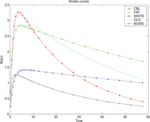
Kinetic behavior used for each one of the structures in the images and standard deviation of noise.
The following procedures Eqs. (11-14) were used for generation of simulated uncorrelated Gaussian, correlated Gaussian and uncorrelated Poisson noise.
If γ is a 2D Gaussian filter of size [5 x 5] with σ of size 2 then correlated Gaussian noise v is defined as 2D convolution (⊗) of the 2D Gaussian distributed random noise fN with mean zero and variance one and the defined Gaussian filter γ.
If Xi refers to 2D image matrices of size [128 x 128], i = (1,2,3,...,24), containing values of four different objects with different kinetics (x1, x2, x3, x4) and background, ρ f refers to a 2D point spread function defining the image resolution, c is a constant for modulating the magnitude of the noise and yi refers to the kinetics of the noise. Then a 2D image Xi with additive, correlated and Gaussian distributed random noise is defined as:
where is each pixel in original image with applied point spread function. Eq. (13) has been employed for creating uncorrelated Gaussian distributed random noise.
For creating Poisson (Eq. 14) distributed noise Samal’s [39] formulation has been employed with a point spread function included in this equation. A 2D image X p containing uncorrelated Poisson distributed noise is defined as:
Synthetic images containing different magnitudes of the additive Gaussian or Poisson distributed noise have been studied. Fig. (2) shows the input images containing uncorrelated Gaussian distributed noise.
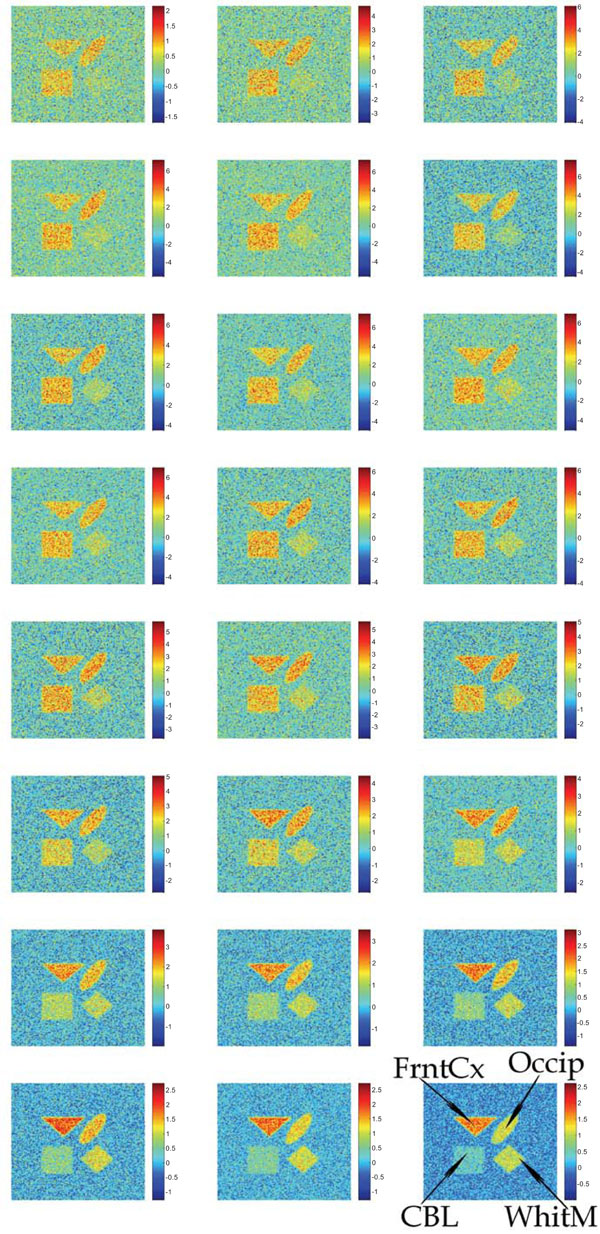
Synthetic images containing different magnitudes of additive and uncorrelated Gaussian noise. The sequence starts in the upper left corner and ends in the lower right corner.
Signal to Noise Ratio (SNR)
As a parameter to define the image quality after application of PCA or ICA, we used the SNR. Here, the definition of SNR from Sonka [51], Eq. (15), was used where signal is defined as the sum of squared values of the pixels within an outlined ROI identifying the objects. The noise is defined as the sum of squared values of the pixel deviation from the mean within an outlined ROI covering the same structure in the image. Eq. (16) indicates the definition of the signal and Eq. (17) indicates the definition of noise for the whole imaging sequence.
where signal
where
and noise
where
For the calculation of the signal and for the noise for each structure we used a mask that covered the inside (minus a number of pixels from the edge) of the structure in the image, ensuring that none of the background or surrounding was included in the mask. SNRs were calculated and illustrated, based on highest ratios within all PC(s) or IC(s) for each part of the study.
Pre-Normalization Methods
In the present study four types of pre-normalization methods were utilized on the data before application of analysis methods and the results were compared with those without pre-normalization.
The first pre-normalization we named background noise pre-normalization, “nor1”, which is an improved version of the method introduced by Pedersen et al. [14]. Distinct from the suggested approach by Pedersen et al. [14], this method is based on dividing the value of each pixel k in a single image i by the standard deviation of the noise calculated from an outlined masked area in the background of each one of the images (slice wise). The reason for using this mask was to cover pixels containing the noise from different positions in the background within the image for better estimation of the standard deviation.
The pre-normalization was performed according to Eq. (18),
where Xik refers to a new value of the pixel k of image i and xik refers to the original value of the corresponding pixel and Si refers to standard deviation of pixels within the mask. This method would normalize for different levels of noise in the imaging sequence, if the noise magnitude was the same all over each image field.
The second proposed method was named “pois” pre-normalization. This method is based on dividing the value of each pixel k in a single image by the square root of the absolute value of the same pixel in the image i and is based on the assumption that the noise variance in each pixel is proportional to the value in this pixel.
Xik denotes the new value of the pixel after applying normalization. This method would normalize for noise if it in each pixel were Poisson distributed both within and in-between images.
The third pre-normalization method is known as whitening, ”whit” and is part of the concept in ICA. This method starts by centering the pixel values meaning that the mean of the pixel values is set to zero followed by a scaling in which the variance of the pixel values is set to one.
where Xnj refers to transformed image and Xj refers to original image j as a vector containing the pixel values and refers to the mean of the vector and N refers to the number of elements in the vector Xj.
In this study we propose a new pre-normalization method denoted as “mixp”, which is based on following steps:
a. Removal of Negative Values
PET images contain negative pixel values in random positions within the images, predominantly in areas with low radioactivity such as outside the object but also sometimes within the object. This is due to filtering of the projections, scatter and random subtraction, which are part of reconstruction algorithm. These negative values are related to noise and hence independent of the values in the same positions in other planes or frames. We declare each one of the negative pixel values within the image as a pixel containing noise. We then treat each one of the negative pixel values independent of other pixels by taking the absolute value of the value of the divided by its square root. Hence, each pixel j in the single image i that contained a negative value Xij obtains new value,
b. Background Noise Pre-Normalization
This method “nor1” was utilized using Eq. (18).
c. Reference Region Pre-Normalization
Reference region pre-normalization was based on dividing the value of each pixel j in a single image i by the mean value of the pixels within a drawn ROI, masking the chosen reference region in each frame (Eq. 22). A reference region is defined as a region, where there is no specific tracer binding. In our synthetic study, the structure “CBL” was used as reference region.
Performing the reference region pre-normalization damps the values of the pixels representing regions with similar kinetic behavior as the reference region and at the same time enhances the contrast of the areas deviating from the reference region.
RESULTS
PCA on Images with Gaussian Noise
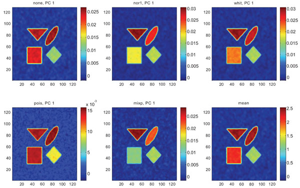
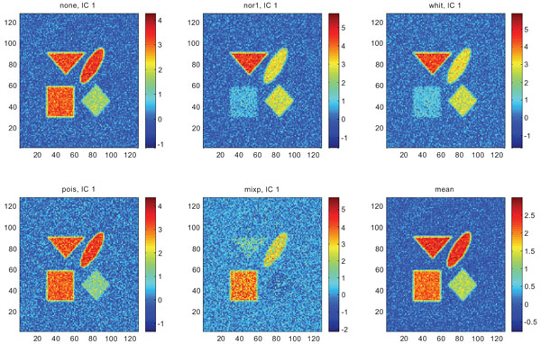
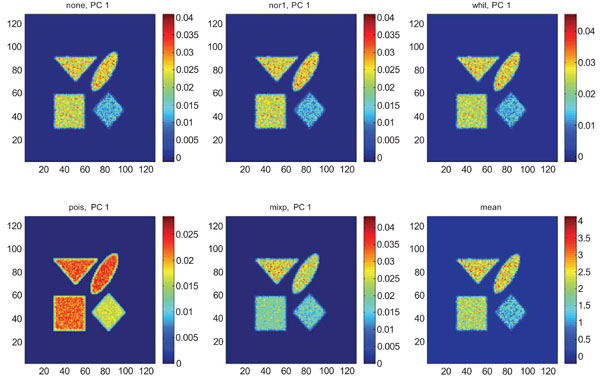
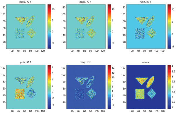
Figs. (3-5) show the results from applying PCA on synthetic images containing uncorrelated Gaussian noise and using different types of pre-normalization methods. The mean image and PC1 images generated with none or “pois” normalization were similar in their features, with highest values in frontal, occipital and CBL structures and lower signal in white matter. The other three normalization methods were also similar in-between them, with highest signal in frontal and occipital structures and lower in CBL and white structures. The “mixp” additionally discriminated between frontal and occipital structures and enhanced the discrimination to CBL and white.
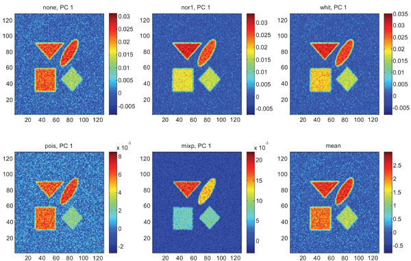
PC1 images obtained after application of PCA on synthetic images containing uncorrelated Gaussian noise and generated utilizing different pre-normalization methods. Upper left shows PC1 image without any pre-normalization, upper middle the “nor1” and upper right the “whit” pre-normalization methods. Lower left shows PC1 image using the “pois” and lower middle the “mixp” pre-normalization methods. Lower right shows mean image.
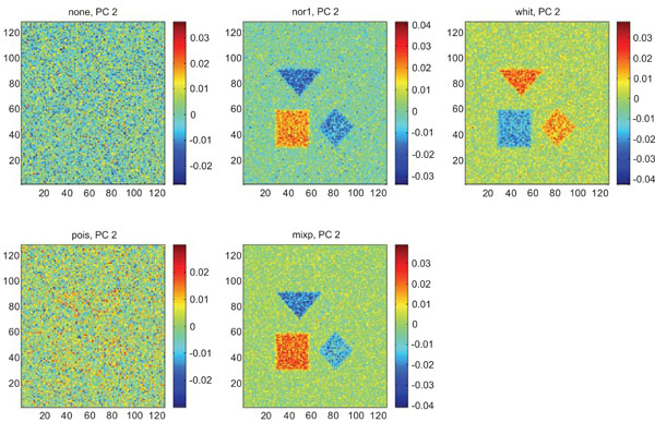
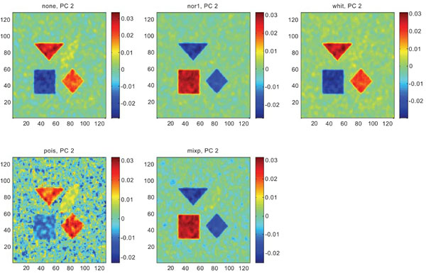
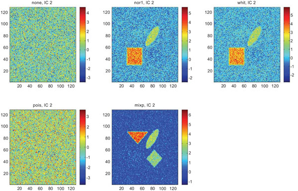
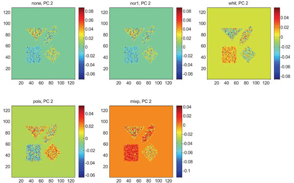
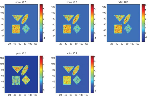
PC2 images obtained after application of PCA on synthetic images containing uncorrelated Gaussian noise. Upper left shows PC2 image without any pre-normalization, upper middle the “nor1”, upper right the “whit”, lower left the “pois” and lower middle the “mixp” pre-normalization methods.
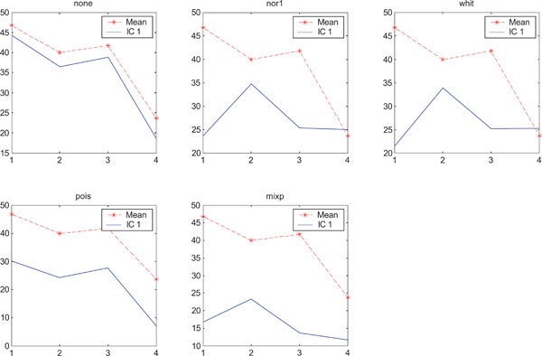
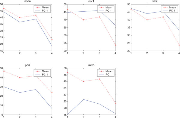
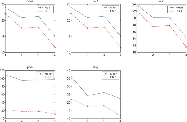
SNR values for the corresponding structures in first principal component (PC1). Images contain uncorrelated Gaussian noise and are generated utilizing different pre-normalized methods and compared with mean image. Each point of the curves representing SNR values for each one of the structures in both mean image (dash-star) and pre-normalized image (solid curve).
The PC2 images with none or “pois” normalization failed to further discriminate between structures whereas the other three normalization methods delineated the structures except occipital.
In rank order the “nor1” and “whit” pre-normalization gave the highest SNR compared to the mean image and “none”, “pois” and “mixp” gave lower SNR than the average image.
Figs. (6-8) show the results from applying PCA on synthetic images containing correlated Gaussian noise and using different types of pre-normalization methods. The mean image and PC1 images generated with none, “nor1”, “whit” and “pois” normalization, were similar in their features to that obtained applying “none” and “pois” pre-normalization on images containing uncorrelated Gaussian noise with highest values in frontal, occipital and CBL structures and lower signal in white matter. The “mixp” discriminated between frontal and occipital structures and enhanced the discrimination to CBL and white. CBL is extracted and separated in PC2.
PC1 images obtained after application of PCA on synthetic images containing correlated Gaussian noise and generated utilizing different pre-normalization methods. Upper left shows PC1 image without any pre-normalization, upper middle the “nor1” and upper right the “whit” pre-normalization methods. Lower left shows PC1 image using the “pois” and lower middle the “mixp” pre-normalization methods. Lower right shows mean image.
PC2 images obtained after application of PCA on synthetic images containing correlated Gaussian noise. Upper left shows PC2 image without any pre-normalization, upper middle the “nor1”, upper right the “whit”, lower left the “pois” and lower middle the “mixp” pre-normalization methods.
SNR values for the corresponding structures in first principal component (PC1) synthetic images. Images contain correlated Gaussian noise and are generated utilizing different pre-normalized methods and compared to the mean image. Each point of the curves representing SNR values for each one of the structures in both mean image (dash-star) and pre-normalized image (solid curve).
PC1 images obtained with applied “pois” pre-normalization gave the highest SNR compared to the mean image. The “none”, “pois” and “whit” gave similar results than average image and “mixp” gave lower SNR than the average image.
The PC2 images with applied pre-normalization using all methods delineated the structures with different SNR values, except occipital in “nor1” and “whit”.
ICA on Images with Gaussian Noise
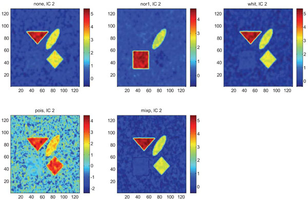
Figs. (9-11) represent the result of applying ICA on synthetic images containing non-correlated Gaussian distributed noise using different types of pre-normalization methods. Also with ICA, none and “pois” showed the same imaging of the structures in IC1 as shown above with PC1, with similar values for frontal, occipital and cerebellum and lower values in white. “nor1” and “whit” gave similar results with highlighting frontal followed by equal imaging of occipital and white and “mixp” gave results? with highlighting cerebellum, occipital in IC1 images and frontal and occipital followed by white in IC2 image.
IC1 images obtained after application of ICA on synthetic images containing uncorrelated Gaussian noise and generated utilizing different pre-normalization methods. Upper left shows IC1 image without any pre-normalization, upper middle the “nor1” and upper right the “whit” pre-normalization methods. Lower left shows IC1 image using the “pois” and lower middle the “mixp” pre-normalization methods. Lower right shows mean image.
IC2 images obtained after application of ICA on synthetic images containing uncorrelated Gaussian noise. Upper left shows IC2 image without any pre-normalization, upper middle the “nor1”, upper right the “whit”, lower left the “pois” and lower middle the “mixp” prenormalization methods.
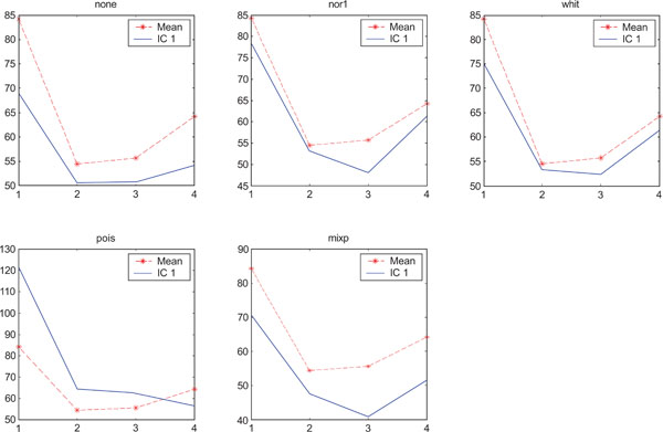
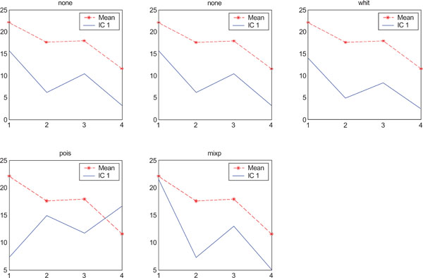
SNR values for the corresponding structures in first principal component (IC1) synthetic images. Images contain uncorrelated Gaussian noise and are generated utilizing different pre-normalized methods and compared to the mean image. Each point of the curves represents SNR.
The IC2 images with none and “pois” normalization only showed noise, whereas “nor1”, “whit” and “nor1” showed CBL and occipital and “whit” showed highest in frontal followed by occipital and white. The SNR were inferior to mean image using different types of pre-normalization methods.
When performing ICA on images with correlated Gaussian noise, the results were improved compared to the result obtained on images with uncorrelated Gaussian noise. SNR were lower compared to average image except on images with applied “pois” pre-normalization method whereas not for structure WhitM as shown in Figs. (12-14).
IC1 images obtained after application of ICA on synthetic images containing correlated Gaussian noise and generated utilizing different pre-normalization methods. Upper left shows IC1 image without any pre-normalization, upper middle the “nor1” and upper right the “whit” pre-normalization methods. Lower left shows IC1 image using the “pois” and lower middle the “mixp” pre-normalization methods. Lower right shows mean image.
IC2 images obtained after application of ICA on synthetic images containing correlated Gaussian noise. Upper left shows IC2 image without any pre-normalization, upper middle the “nor1”, upper right the “whit”, lower left the “pois” and lower middle the “mixp” prenormalization methods.
SNR values for the corresponding structures in first principal component (IC1) synthetic images. Images contain correlated Gaussian noise and are generated utilizing different pre-normalized methods and compared to the mean image. Each point of the curves represents SNR.
PCA on Images with Poisson Noise
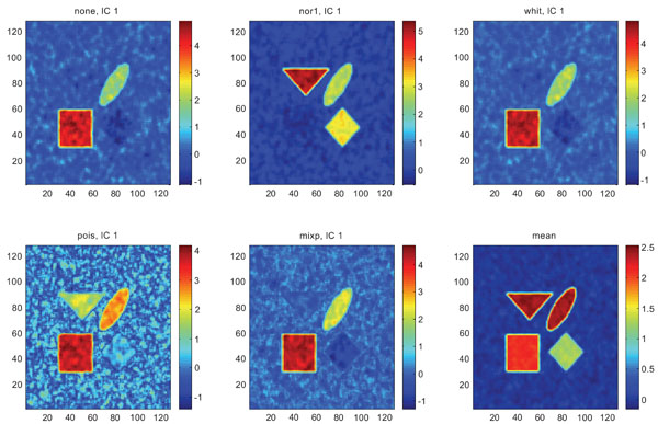
When applying PCA on images generated with Poisson noise (Figs. 15-17), the optimal discrimination of the structures in PC1 images were seen with “pois” normalization. The other pre-normalization methods gave relatively similar images with equally high values in the structures except white.
PC1 images obtained after application of PCA on synthetic images containing uncorrelated Poisson noise and generated utilizing different pre-normalization methods. Upper left shows PC1 image without any pre-normalization, upper middle the “nor1” and upper right the “whit” pre-normalization methods. Lower left shows PC1 image using the “pois” and lower middle the “mixp” pre-normalization methods. Lower right shows mean image.
IC2 images obtained after application of ICA on synthetic images containing uncorrelated Poisson noise. Upper left shows IC2 image without any pre-normalization, upper middle the “nor1”, upper right the “whit”, lower left the “pois” and lower middle the “mixp” prenormalization methods.
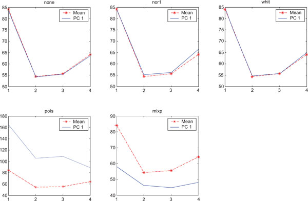
SNR values for the corresponding structures in first principal component (PC1) synthetic images. Images contain uncorrelated Poisson noise and are generated utilizing different pre-normalized methods and compared to the mean image. Each point of the curves representing SNR values for each one of the structures in both mean image (dash-star) and pre-normalized image (solid curve).
PC2 images identified all structures, primarily because of high noise in the structures and lack of noise in the surrounding. SNR was improved with all methods as compared to the mean image especially using “pois” pre-normalization method in which the ratio is 5 times higher compared to the mean image.
ICA on Images with Poisson Noise
The application of ICA on images with Poisson noise (Figs. 18-20) seemed in general to place information rather in IC2 images than IC1 images which were very noisy. Additionally none of the methods was able to highlight the structures of greatest interest, frontal and occipital. The SNR was inferior for all structures and methods as compared to the mean images, except structure WhitM with “pois” normalization.
IC1 images obtained after application of ICA on synthetic images containing uncorrelated Poisson noise and generated utilizing different pre-normalization methods. Upper left shows IC1 image without any pre-normalization, upper middle the “nor1” and upper right the “whit” pre-normalization methods. Lower left shows IC1 image using the “pois” and lower middle the “mixp” pre-normalization methods. Lower right shows mean image.
PC2 images obtained after application of PCA on synthetic images containing uncorrelated Poisson noise. Upper left shows PC2 image without any pre-normalization, upper middle the “nor1”, upper right the “whit”, lower left the “pois” and lower middle the “mixp” prenormalization methods.
SNR values for the corresponding structures in first principal component (IC1) synthetic images. Images contain correlated Gaussian noise and are generated utilizing different pre-normalized methods and compared to the mean image. Each point of the curves represents SNR.
DISCUSSION
The main scope of this work was to explore the application of two well-known, unsupervised multivariate image analysis tools, namely PCA and ICA, on a dynamic sequence of PET images. We wanted to study the performance of these two methods on PET images where the behavior of the noise is different compared to studies on other medical imaging modalities such as CT, MRI, fMRI and EEG etc. We aimed to explore these tools’ capability to extract signals from noise in these types of noisy images to suggest one method to be used in clinical settings. Since clinical PET images contain such complicated structures and kinetic behavior, we selected to use simulated images where we could better control structure and noise and also analyze the results.
There is not one single entity which would describe the optimal imaging of complex kinetic/biological behaviors. We would desire a good imaging of structures, a good discrimination in-between structures with different characteristics and we would like these tasks to be performed with the optimal SNR.
In contrast to previous studies e.g. [31] and [33], we wanted to utilize these methods on noisy PET images to investigate whether the pre-normalization of the input data can improve their performance. The reason was that we believe that PCA is a reliable multivariate technique, but only if the input data is handled properly since PCA is “blind” to the difference between variance created by signal and created by noise. Therefore, different types of pre-normalization methods were proposed and investigated.
One of the ambitions in applying different pre-normalization methods was to determine the pre-normalization method in which the variance of the noise in the sequence of images becomes as stable as possible in the time sequence (frames). This would allow PCA to detect fluctuations in the signal and not be guided by the noise. In other words by applying pre-normalization, the input data would be transformed to data where the variance of the values are more stable during the time interval and at the same time the signal strength would be preserved as much as possible before applying PCA. In parallel we wished to explore if the same pre-normalization of input data would affect the performance of the ICA on noisy PET data.
To reach the goals of this study, we generated synthetic PET images containing uncorrelated and correlated noise where the signal vs. noise behavior could be controlled yet qualitative vs. quantitative results could be generated. The reason for employing correlated noise in the simulation study was to explore if the correlation of the noise affected the performance of these methods or not. Synthetic image sequences with different high noise magnitudes were studied to validate the performance of the suggested methods and to explore if the employed pre-normalization method could damp the effects of the noise in derived images.
Because of the large interest in the potential use of the amyloid binding tracer PIB, we selected to generate structures in the simulated images which followed the kinetic behavior of PIB in these structures and generated a noise which simulated that of a PIB imaging sequence with respect to magnitude.
Since images reconstructed with different reconstruction methods would differ in their noise characteristics, we included in the simulation’s noise which was globally similar across the image and noise which had a Poisson distribution related to the magnitude in each pixel. Finally we included correlation of noise by convolution.
Application of PCA generated relatively similar results, with some minor differences, on the images with correlated and uncorrelated Gaussian noise characteristics when input data were not pre-normalized. However, clear differences were noticeable using different noise characteristics (Gaussian vs. Poisson) when input data were not handled with proper pre-normalization method. Improvement of performance of PCA was observed on images containing Poisson distributed noise applying different pre-normalization method especially “pois”.
The best qualitative illustration were observed on PC1 images especially on images containing correlated Gaussian noise but the best quantitative results were obtained on images containing Poisson distributed noise when input data were handled by a proper pre-normalization.
Hence “nor1”, “whit”, “pois” and “mixp” gave PC1 images, which had a desired enhancement of the most interesting structures frontal and occipital cortex. These normalization methods also succeeded to discriminate in-between the structures in PC2 images except “pois” applied on images containing un-correlated Gaussian noise. The “nor1” and “mixp” normalizations also created PC1 images with improved SNR as compared to the mean images and in some cases separated structures in different components such as in images containing correlated Gaussian noise. An overall slight preference for the “mixp” and “pois” normalization was identified when reviewing all image results.
ICA with “nor1”, “pois” and “mixp” pre-normalization also seemed to perform relatively well. It was noticeable that the SNR calculated for the WhitM was higher compared with mean images when performing “pois” pre-normalization on both uncorrelated and correlated compared with other structures. One possible reason might be that the kinetic behavior of the WhitM did not vary as much as the other structures. However ICA did not reach the improvement in SNR as PCA did. Furthermore ICA seemed to have a tendency under some conditions to shift over information from IC1 to other independent components and to be more sensitive to the level of noise.
CONCLUSIONS
The results from this study showed that PCA is a more stable technique compared with ICA and creates better results both qualitatively and quantitatively especially when “mixp” pre-normalization was used. Applying pre-normalization does not improve the performance of the ICA for quantitative measurements dramatically.
PCA can extract the signals from the noise rather well and is not sensitive to magnitude and correlation likewise type of noise, when the input data are correctly handled by a proper pre-normalization. It is important to note that PCA as inherently a method to separate signal information into different components could still generate PC1 images with improved SNR as compared to mean images.
PC1 and IC1 images may lose the quantitative values and relations within the images, meaning that the quantitative difference between different structures in the image will not be the same as in the real case. Future work could suggest how it is possible to get quantitative measurements out of PC and IC images.
ACKNOWLEDGMENTS
The authors wish to thank Dr. Azita Monazzam, for beneficial scientific discussions.