All published articles of this journal are available on ScienceDirect.

Overview of Recent Advancement in Ultrasonic Imaging for Biomedical Applications
Abstract
This paper discusses the application of acoustic microscopy to the detection of cancerous cells. Acoustic microscopy is a well-developed technique but the application to biological tissues is challenging. Acoustic microscopy images abnormality based on the difference in the acoustic impedance from the background. One of the difficulties in the biomedical applications is that since both normal and abnormal cells consist of mostly water, their acoustic impedance is quite close to each other. Consequently, the contrast of the image tends to be low. Another issue is concerning the spatial resolution. For higher resolution, the use of a short wavelength is essential. However, since the attenuation of an ultrasonic signal increases quadratically with the frequency, the reduction in the wavelength compromises the image quality. The present paper addresses these issues and describes various techniques to overcome the problems.
1. INTRODUCTION
The diagnosis of cancerous cells is one of the most essential steps in cancer treatment. Currently, biopsy followed by pathological examination based on optical microscopy is the most prevailing technique. Although this methodology is well established, it is not almighty. The main limitation of biopsy is the problem of sampling error. Diagnosis based on a small number of samples does not necessarily represent the pathological process of the entire organ. This is particularly true when there is a localized pathological process in the organ. Increase in the number of specimens may reduce the sampling error. However, it requires the removal of a large volume of tissues from the patient who is suffering from the disease, and therefore unrealistic. An optical microscopic examination following biopsy has an intrinsic problem as well. Conventionally, the preparation of microscopic specimens involves a staining and/or chemical fixing process, which normally kills the cells. Consequently, the examination is unable to reveal the phenomena that only living cells indicate, and that can be essential to understand the behavior of the cancerous cells and hence to determine the treatment. In addition, it takes at least a week to prepare the specimen. A technique capable of visualizing in-situ cellular details in multiple areas is much more desirable.
In this regard, acoustic microscopy [1-6] is quite advantageous, as it is capable of visualizing cellular abnormalities in living cells [7]. With the operation frequency 1 GHz or higher, a spatial resolution of submicron is achievable [8]. Often it is of extreme importance to understand the pathological behavior of cancerous cells in the living organ because it indicates the prognosis of the disease. In addition, since the technique relies on acoustic waves passing through the subject, it may allow obtaining information along the depth of the subject via measurement of mechanical properties (e.g., loss factor and modulus) of tissues [9]. It is unnecessary to make a thin specimen for diagnosis. In principle, an in-vivo application similar to a recent invention of multimodal endoscope method [10] is possible. As another example of in-vivo application of acoustic technology, Burns et al. have invented a non-invasive method to measure the pH value of a fluid in a living body [11].
With these advantages, however, acoustic microscopy has intrinsic difficulties when applied to biological systems [12-16]. As explained later in this paper, acoustic microscopy detects abnormalities based on the difference between the propagation of the acoustic wave in the inclusion and in the surrounding entities. This difference is called the contrast. It is a well-established method used in various engineering applications [17-19] such as nondestructive evaluation of solid objects [20-26]. In most cases, the contrast is made based on the difference in the propagation speed of the acoustic wave in the abnormality (the difference in the acoustic impedance) [27, 28]. However, in most biological systems, the acoustic wave velocity is quite close to that in water, which is not surprising because biological cells are constituted mostly by water [29]. Consequently, the contrast is essentially low. It is also possible to make a contrast based on the amplitude or the difference in the transmission between the abnormality and the surrounding entities. However, since attenuation of acoustic signal increases quadratically in proportion to the frequency [30], it becomes difficult to use high frequency for thick specimens. Since the wavelength is inversely proportional to the frequency, this means that the spatial resolution is reduced. There is always a trade-off between the spatial resolution and the thickness of the subject.
The aim of this paper is to give an overview of acoustic microscopy in its application to biomedical systems. After a brief description of the history and principle of acoustic microscopy, its applications to specific cancer cells are discussed based on previous experimental data1.
2. HISTORICAL BACKGROUND
The first attempt to study microstructures of biological specimens with a mechanical scanning acoustic transmission microscope was made by Lemons and Quate [8]. Maev et al. [31] extended this technique and intensively applied it to various biological objects. For their type of a system, a specimen is located between the lenses, so that the thickness of the specimen is limited. Therefore, this technique did not receive widespread attention.
There are quite a few publications for investigating living cells as well as thinly sliced tissue with SAM [32-50]. However, few articles have been published for a tissue including cancer cells or tumors [51-57]. The research has been conducted with liver, prostate and eye cells, performed with frozen or formalin-fixed slices, and it was demonstrated that acoustic images distinctly and precisely reveal abnormal portions in the tissues.
SAM has been applied in medicine and biology by Tohoku University since 1980 [58, 59]. One of the arguments for using SAM in medicine is that SAM can be applied for intra-operative pathological examination since it does not require a special staining technique. A group of researchers at the University of California in Irvine determined that a resolution corresponding to a frequency of 600 MHz was sufficient to render a microscopic diagnosis [60, 61]. Saijo, Y., et al. showed that SAM can also classify the types of cancer in the stomach [62] and kidney [63] by quantitative measurement of ultrasonic attenuation and the sound speed at 200 MHz.
Ultrasonic data obtained with high-frequency SAM can be used for assessing reflectability or texture in clinical echo-graphic imaging. It has been shown that the calculated reflection and clinical data were matched in the myocardium [64]. Chandraratna et al. also assessed the echo-bright area in the myocardium by using 600 MHz SAM [65]. The values of attenuation and sound speed in six types of tissue components of atherosclerosis were measured by 100~200 MHz SAM [66]. As the term arteriosclerosis means hardening of the artery, atherosclerotic tissues have been known to increase in stiffness or hardness in the development of atherosclerosis. Assessment of the mechanical properties of atherosclerosis is important, in addition to determining the chemical components of the tissue. The composition of atherosclerosis is defined as the collagen fibers, lipid and calcification in the intima, the smooth muscle and elastic fiber in the media, and the collagen fibers in the adventitia, respectively. The variety of the degree of staining for optical microscopy indicates that the collagen content or the chemical property is not homogeneous in fibrotic lesions of the intima.
3. PRINCIPLE OF ACOUSTIC MICROSCOPY
3.1. Acoustic Reflection Microscope
In this section, a brief description of an acoustic microscopic technique known as the acoustic reflection microscopy [1] is given. In this technique, the incoming acoustic beam is focused by an acoustic lens, and converges as it propagates through the system towards the specimen. The beam is reflected at various boundaries of different media in the system, and propagates back to the source. Since the acoustic beam is focused, the wave-front curvature of the returning wave varies as a function of the distance from the specimen. A curved wavefront can be expressed as a summation of a series of plane waves oriented in different directions. In the Fourier (spatial frequency) domain, different curvatures correspond to different spatial frequency components. Therefore, signals from different depth in the specimen can be distinguished from one another as different frequency components. The method is also called the angular spectrum method [67, 68].
The angular spectrum method enables us to perform a quantitative analysis. When the acoustic wave is a Gaussian beam, which is often the case, the analysis becomes quite simple in the Fourier domain. The principle of operation can be summarized as follows. Since the angle of diffraction depends on the wavelength, the curvature of the wavefront of an acoustic wave at a given distance from the source varies as a function of the wavelength. The phase velocity of an acoustic wave, which is the product of the frequency and wavelength, is determined by the medium that the wave is transmitted through. Consequently, when a diverging or converging acoustic wave consisting of various frequencies is emitted from the same source and reflected back towards the source, the transverse, spatial profile of the returning beam at a given plane normal to the axis representing the depth depends on the reflecting surface’s profile and the elastic property of the medium that the wave is transmitted through. If either the reflecting surface or the medium between the reflecting surface and the incident surface (the surface where the returning beam is detected) has non-uniformity, it changes the propagation of the wave and the result is observed as a contrast in the final image. If the reflecting surface is close to the focal plane of the acoustic wave and at the rear surface of the specimen, the acoustic wave propagates only through a portion of the specimen (because the cross-sectional area of the acoustic beam inside the specimen is small); the returning beam contains information of that portion of the specimen. By scanning the acoustic wave transversely, we can form a whole view of the specimen.
Fig. (1) illustrates a typical setup of the technique called acoustic reflection microscopy with the angular spectrum method in the pulsed wave mode [1]. The acoustic transducer emits a plane acoustic wave at plane 0. Here is the acoustic field whose physical meaning will be clarified below, the subscript 0 denotes the plane and the superscript indicates the propagation direction of wave at the plane where "+" represents the forward going beam (traveling in the positive direction) and "-" the returning beam. The definitions of the superscript and subscript are common to all planes. The curved shape of the bottom surface of the buffer rod makes the rod be acting as a converging acoustic lens. Planes labeled 1 and 2 represent the back and front focal planes of the acoustic lens. (They are not at the same distance from the lens because the different media are involved.) Plane 3 is at the front surface of the cover of the container holding the specimen. Plane 4 is at the back surface of the cover that is the interface between the cover and the front surface of the specimen. Plane 5 is the interface between the back surface of the specimen and the front surface of the substrate.
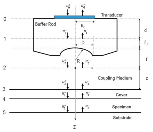
In the pulsed mode operation, the transducer emits an acoustic wave pulse. The returning beam is received by the transducer through an electric gate with a certain width. By adjusting the delay and width of the gate (i.e., the position and duration on the time axis), it is possible to receive the acoustic wave reflected at a certain position along the -axis.
3.2. Angular Spectrum Representation
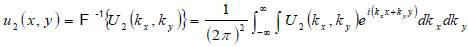
This section briefly describes how to decompose a complicated wavefront into an angular spectrum of plane waves by the Fourier transformation [69-71]. Suppose that a monochromatic wave, propagating along z-axis, is incident at the z1 plane. The complex field of the wave is given by u1(x,y) with e-iωt time dependence suppressed. Then, the angular spectrum in the plane is given by the following equation:
 |
(1) |
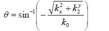
With Eq. (1), we can decompose the acoustic field u1(x,y) into plane wave components of the form e-i(kxx+kyy) having an amplitude U1(kx,ky). Here, e-i(kxx+kyy) represents a unit amplitude plane wave incident on the z1 plane with an angle
 |
(2) |
 |
(3) |
where ω is the angular frequency, and V0 is the sound velocity.
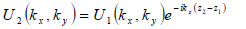
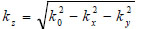
The angular spectrum at another plane, z2, can be found by multiplying U2(kx,ky) by eikz(z2-z1) where 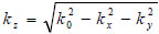 to give
 |
(4) |
Note that for 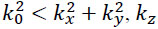 is purely imaginary and the corresponding plane wave is evanescent.
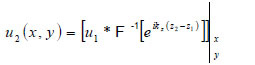
With the spectrum in this form, the complex field at z2 can be determined by inverse Fourier transform
 |
(5) |
Note that 
In this space, Eq. (4) can be written as
 |
(6) |
where “*” signifies the convolution operation.
If so-called paraxial approximation is used, the expression can be simplified, since we have 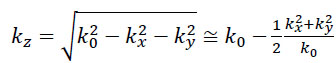 for
for 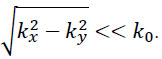 . Therefore, we can approximate eikz(z2-z1) as follows:
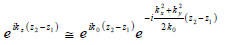 |
(7) |
The first exponential factor in Eq. (7) is an overall phase retardation suffered by any component of the angular spectrum as it propagates from z1 to z2. The second exponential factor is phase dispersion with a quadratic frequency dependence on the spatial angle.
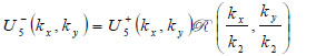
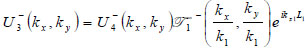
Let a second region be introduced separated from the first region by a plane boundary at z3. If a plane wave of the form U3(kx,ky)ei{kxx+kyy+kz(z-z3)} is incident on this boundary, there will be a reflected plane wave of the form U '3(kx,ky)ei{kxx+kyy+kz(z-z3)}. Suppose that the reflectance function  of the boundary is known. The function relates U3(kx,ky) to U '3(kx,ky) as follows [70]:
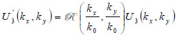 |
(8) |
3.3. Contrast Theory for SAM (Pulse-Wave Mode)
Below an expression of the contrast of a specimen is derived [67]. The transducer excites a uniform field (i.e., u +0 (x,y)) when a unit voltage is applied at its terminals. The transducer output voltage, represented as a function of z, is the integral of the incident field (i.e., u-0 (x,y)), over the cross-sectional area of the transducer. Here it is assumed that the acoustic beam is approximated as a Gaussian beam.
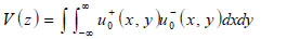 |
(9) |
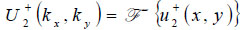
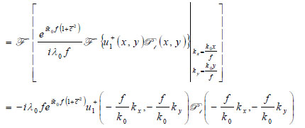
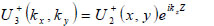
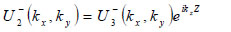
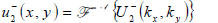
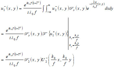
With the knowledge of the distance from the plane where the transducer is placed and the back focal plane (Plane 1), the acoustic field at Plane 1 u +1(x,y) can be computed easily in the Fourier domain. Once u-1(x,y) is known, the acoustic field at each critical plane can be computed as follows:
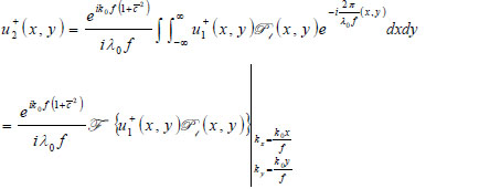 |
(10) |
where  is the wave number in the coupling medium (i.e., de-ionized water), λ0 is the wavelength of the coupling medium, f is the focal length of the lens,
  is the ratio of the sound velocity in the coupling medium to that in the solid (i.e., material of the buffer rod such as fused quartz), and
  is the pupil function expressed as the following equation.
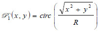 |
(11) |
where R is the radius of the pupil function of the lens.
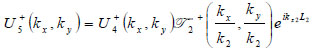
Propagation of the wave beyond the focal plane is easily calculated if the angular spectrum representation is utilized.
 |
(12) |
 |
(13) |
 |
(14) |
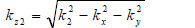
The lens is adjusted to focus the forward going acoustic beam on the front surface of the substrate through the cover and the specimen so that the returning beam reflected on the substrate surface is maximized.
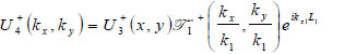 |
(15) |
 |
(16) |
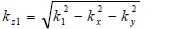
where  is the transmittance function within the cover,
  is the wave number in the cover, and λ1 is the wavelength in the cover.
 |
(17) |
 |
(18) |
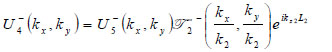
where  is the transmittance function within the specimen,
  is the wave number in the specimen, and λ2 is the wavelength in the specimen.
 |
(19) |
 |
(20) |
 |
(21) |
 |
(22) |
 |
(23) |
 |
(24) |
4. APPLICATIONS TO CANCER CELLS
4.1. Breast Cancer Example
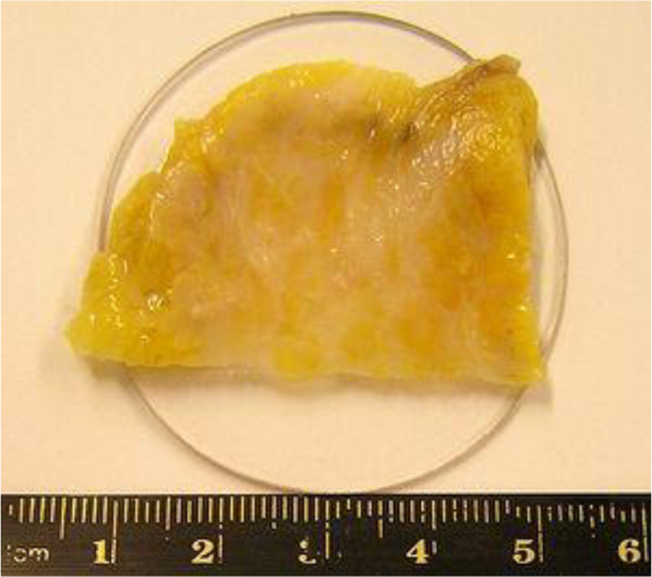
Fig. (2) shows the breast cancer specimen used in this study. It is a 5 mm section of an infiltrating ductal carcinoma of the breast with a rim of normal tissue. Its surface is flat. The tumor in the center has a firmer consistency, and the boundary between the tumor tissue and normal adipose tissue is clearly recognized as illustrated in Fig. (2).
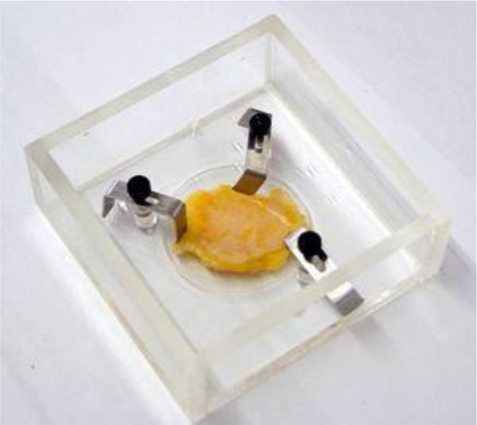
For visualization of cancer tissues in a thick specimen like in this case, it is important to place the specimen on a substrate made of a material having high acoustic reflectivity (acoustic impedance) such as a sapphire (Table 1), so that the acoustic signal is sufficiently strong after the reflection (Fig. 3). The chamber is filled up with a coupling medium ( e.g., water).
An appropriate acoustic lens must be selected in accordance with the thickness of the specimen.
Identification of the correct signal of the reflection from the surface of the cancer tissue is usually the most significant step of this type of experiment. It can be done by monitoring the amplitude of the signal as moving the z-axis of the lens. By selecting the second signal, which is the reflection from the substrate surface (the first signal is the reflection from the surface of the specimen), readjust the z-axis of the lens to maximize the amplitude. Once it is focused, gate the signal and input dimensions along the x- and y-axes ( e.g., 10 mm × 10 mm) for the interested area. It is important to determine an appropriate speed for scanning area of the specimen considering resolution.
| Polystyrene | Z= 2.52 kg/(m2 s)×106 |
| Silica Glass | Z= 13.0 kg/(m2 s)×106 |
| Sapphire | Z= 44.3 kg/(m2 s)×106 |
4.2. Effect of Frequency
Fig. (4) shows an acoustic image of a thickly sectioned normal breast tissue (thickness: 5 mm) with an acoustic lens (SONIX) operating frequency at 50 MHz. Generally speaking, the resolution in the image is limited by the frequency of the acoustic beam; the lower is the frequency the longer is the wavelength compromising the resolution. With the frequency of 50 kHz, the resolution is not necessarily high. However, the darkest spots indicating the ducts of the tissue are clearly observed. The ducts are surrounded by fat cells, which can be seen as a relatively light area. Note that the bright circles are the air bubbles between the tissue and the substrate.
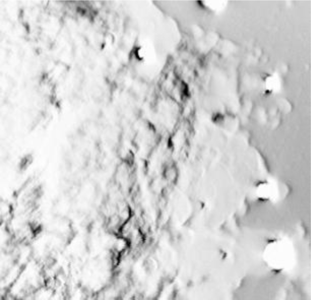
The scanning area of the image is 10 mm × 10 mm, and 50 MHz is the maximum frequency emitted from the acoustical lens to the specimen. The acoustic beam is focused at the interface between the specimen and the substrate.
4.3. Abnormal Tissue
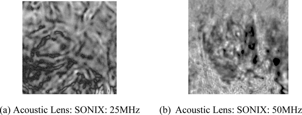
Fig. (5a) is an acoustic image formed with an acoustic lens of frequency at 25 MHz. The image is too unclear to analyze. Fig. (5b) is an acoustic image formed with an acoustic lens of frequency at 50 MHz. This image shows groups of cancer cells. This comparison indicates that to observe the cellular details of the thickly sectioned breast tissue, it is necessary to select an acoustic frequency of 50 MHz or higher.
4.4. Comparison With Optical Image
To understand the acoustic image shown in Fig. (5b), it is necessary to make an observation of the same specimen with an optical microscope. For this purpose, the specimen was included in paraffin and thinly sectioned by a microtome.
Fig. (6) is an optical image of the thinly sectioned specimen and shows a sub-gross image of a high-grade intraductal carcinoma of the breast. The specimen was stained with an Eosin and Hematoxylin and located on a glass slide. Tumor cells are here in blue and fibrous stromal tissues are in pink. Tumor cells are infiltrating normal adipose tissue (clear).

Fig. (7) is an acoustic image of a thinly sectioned breast cancer specimen (not stained) with a thickness of 10 μm, which is scanned with the pulse-wave mode, wherein the scanning area is 20 mm × 20 mm, to compare with the optical image. A 250 MHz acoustical lens (SONIX) is used to form the image.
The portion showing a group of cancer cells (i.e., ductal carcinoma) is magnified (Fig. 8). The darkest spots indicate the calcium in the cells. A 250 MHz acoustic lens (SONIX) is used to form the image and its scanning area is 6 mm × 6 mm.
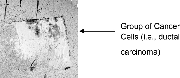
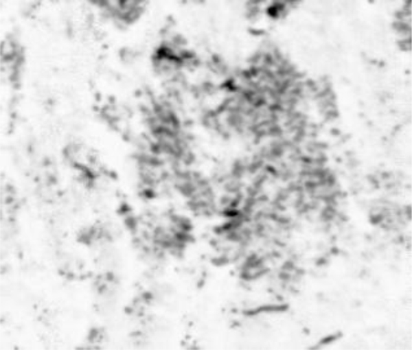
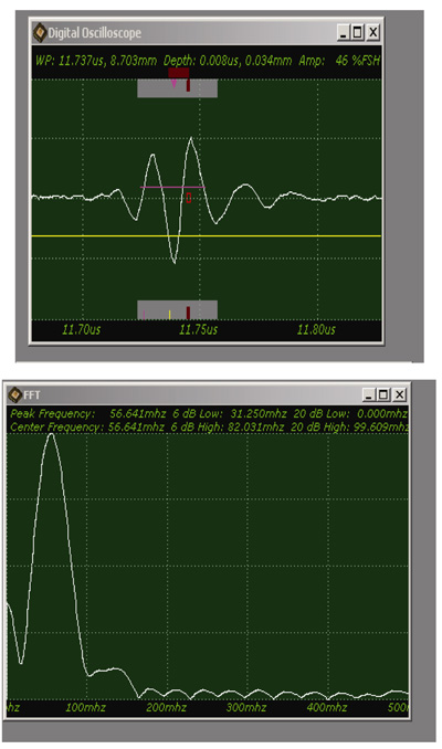
Fig. (9) shows a sample acoustic signal from the thinly sectioned specimen placed on a sapphire substrate. Note that although the acoustic lens emits an acoustic beam having the central frequency of 250 MHz, the frequency of the acoustic beam returned from the specimen is substantially 57 MHz. This is because of the high attenuation in the tissue including groups of cancer cells. It means that emitting a high-frequency acoustic beam is not an appropriate way to form a highly resolved acoustic image in the pulse-wave mode.
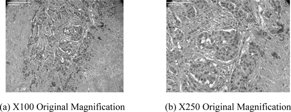
Figs. (10a and b) are higher power optical images of the breast tumor showing infiltrative growth of malignant cells that are seen in irregular nests in the fibrous stroma. Pleomorphic nuclei and frequent mitotic figures indicate a high-grade carcinoma. Figs. (10a and b) confirm that the acoustic image observed in Fig. (5b) is a group of cancer cells.
4.5. Skin Cancer Example
Application to skin cancer is discussed in this section. Being exposed to the body surface, skin cancer is easier than other cancer to apply acoustic waves. The present study was conducted with in-vivo applications in mind. As mentioned in the preceding section, in-vivo application means that the subject is thick and attenuation of the acoustic wave becomes a key issue. In addition to the problem that the attenuation has a quadratic dependence on the acoustic frequency and thereby there is always a trade-off between keeping a strong signal and high spatial resolution, surface roughness degrades the quality of the acoustic image. Below, these issues are addressed with some examples.
4.5.1. Specimen
Fig. (11a) is a thickly sectioned abnormal (melanoma) skin tissue including groups of cancer cells. The thickness of the tissue is 3.0 mm. Fig. (11b) is a thickly sectioned normal skin tissue with the same thickness of 3.0 mm. The images are formed by the digital camera (Olympus). The abnormal tissue has a firmer consistency, is substantially flatter, and has less surface roughness. The tissue includes black, white, and yellow colored portions. The black colored portions have been diagnosed as melanoma carcinoma. The carcinoma area has less surface roughness than the normal sections.
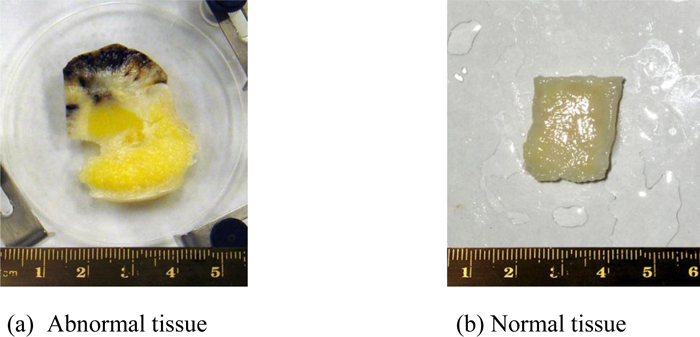
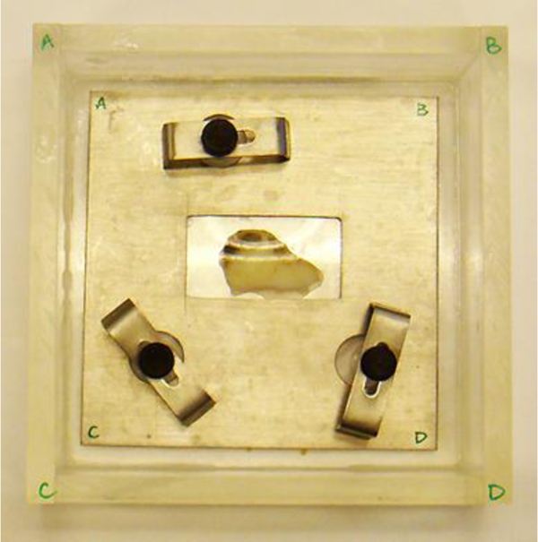
Fig. (12) shows a thickly sectioned melanoma skin tissue specimen located on the surface of a substrate made of c-cut sapphire (acoustic impedance Z= 44.3 kg/(m2 s)×106) with a thin transparent poly-silicone (thickness: 500 μm) cover pressed onto the tissue by a holder made of aluminum. The cover makes the surface of the specimen flat, thereby reducing the effects on the acoustic image caused by surface roughness. The cover also prevents the specimen from floating into the water. The chamber is filled up with a coupling medium (i.e., water).
4.5.2. Optical Image
Figs. (13a and b) are optical images of the thickly sectioned melanoma and normal skin tissues. These images are formed by a Stereoscopic Microscope (Olympus, Model: SZX16). The optical image shows only the surface information of the thick tissues. The surface of the melanoma tissue varies in contrast, which indicates that the specimen has elastic discontinuities. Whereas the normal skin tissue is consistent in contrast, meaning that the internal structure of the specimen is continuous.
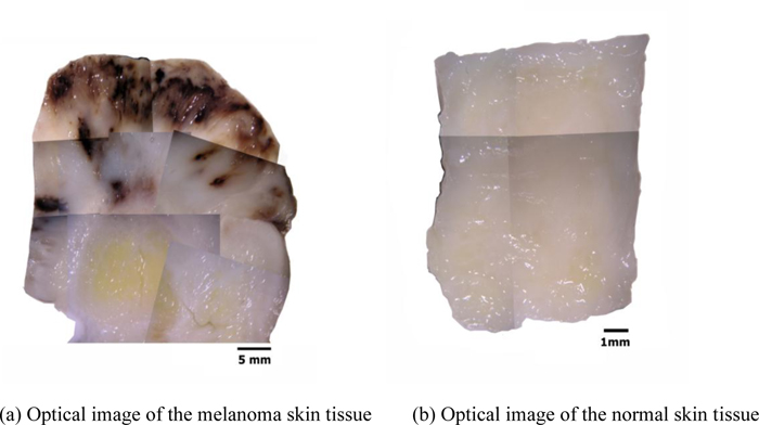
By comparison with the normal tissue, the appearance of the black coloration in the abnormal tissue is evidently recognized as melanoma. The optical image of the abnormal tissue shows that the full extent of the carcinoma tumors spread mostly in the epidermis and the dermis. It also shows that tumors scattered into the hypodermis and appeared around the cartilage, which is present in the yellow zone surrounded mostly by fat. Within this zone, the cartilage is merged with the adjacent supporting tissue containing adipocytes, capillaries and small nerves.
4.5.3. Acoustic Images (C-Scan)
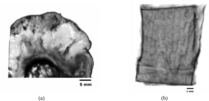
Figs. (14a and b) are acoustic C-Scan images (two-dimensional display of the image of reflected echoes at a focused plane of interest) [72] of thickly sectioned abnormal melanoma and normal skin tissues. The thickness of the specimens is 3 mm, and the input frequency to the acoustic lens (Olympus NDT) is 50 MHz, the maximum frequency for this acoustic system. The acoustic beam is focused at the interface between the specimen and the substrate [z=0 µm or V(0)]. The resolution of the image is limited by the acoustic frequency. The image in Fig. (14a) does not allow us to identify melanoma cancer cells, indicating that an acoustic lens system operating at a frequency higher than 50 MHz is necessary for the analysis of 3.0 mm-thick specimens.
Acoustic properties (i.e., the reflection coefficient, attenuation, and velocity of acoustic wave) and the surface condition (i.e., the surface roughness and discontinuities) of the specimen provide important pieces of information for diagnosis based on acoustic images. It is essential to characterize the specimen for these parameters. For this purpose, analysis of the waveforms, FFT analysis and B-Scan [73] (cross-sectional display over a vertical plane along an axis normal to the plane) need to be performed.
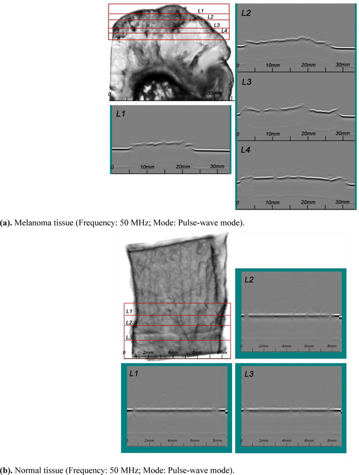
4.5.4. Acoustic Images (B-Scan)
A SAM B-scan image [73] forms a vertical, cross-sectional image of a specimen. Figs. (15a and b) are B-scan images of melanoma and normal skin tissues, showing the surface condition of the respective specimens. They clearly illustrate that the surface of the abnormal tissue is much rougher. The surface structure of the normal tissue is more uniform, consistent, and homogeneous.
4.6. Waveform Analysis (A-Scan) [74]
4.6.1. Attenuation
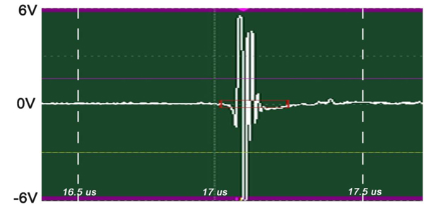
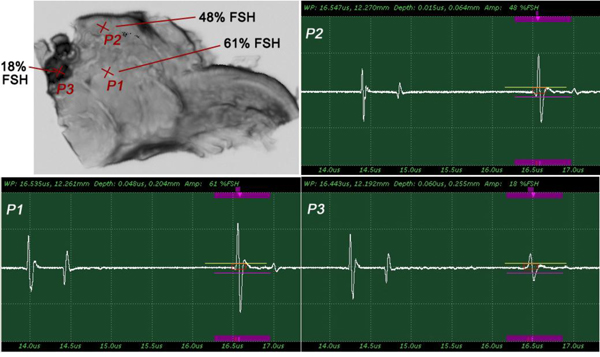
The insertion technique [75] is used to measure the acoustic properties of the different materials. This technique is a relative method, which employs water as the reference to measure the transmission of longitudinal ultrasonic waves through solid media embedded in an aqueous environment (i.e., water). Therefore, the waveform of the wave reflected from the substrate via water was taken as a reference waveform (Fig. 16). In this case, the acoustic beam is focused on the sapphire substrate, and because of the high reflectivity, the reflected signal carries relatively high energy and its waveform has the amplitude of 100% Full-Screen Height (hereinafter called simply “FSH”). The echo amplitudes represent the product of the local scattering strength and the attenuation loss factor, which takes into account scattering in all directions and absorption. Based on the difference, in contrast, three points (i.e., P1, P2 and P3 in Fig. 17) were chosen. The waveforms corresponding to these points are shown in Fig. (17), and their amplitudes of waveforms are shown in Table 2.
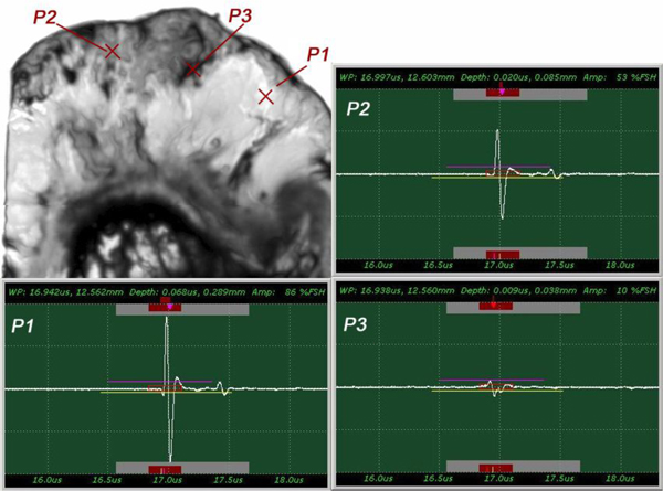
| P1 | A = 86% FSH |
| P2 | A = 53% FSH |
| P3 | A = 10% FSH |
The tissue (see Fig. 17) includes melanoma cancer cells, which were sandwiched between the poly-silicone cover and the sapphire substrate.
The FFTs of P1, P2 and P3 were obtained (Fig. 18) as well as their center frequency and signal loss (Table 3).
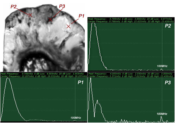
| P1 | fc = 12.207MHz | Δ = 14.111 MHz |
| P2 | fc = 9.766 MHz | Δ = 16.552 MHz |
| P3 | fc = 5.371MHz | Δ = 20.947 MHz |
It can be seen that the frequency of the acoustic beam returned from the thickly sectioned abnormal tissue is less than 15 MHz because of the high attenuation of the tissue including cancer cells. It is concluded that emitting a 50 MHz frequency acoustic beam is not an appropriate way to form a highly resolved acoustic image in the pulse-wave mode.
Since the skin tissues are acoustically transparent, there is no ultrasonic reflection from the surfaces of the tissues. The contrast of the tissues in the acoustic image is primarily generated from the difference in attenuation. From a comparison of the amplitudes of the waveforms, it can be said that the highest attenuation occurs at P1 and the lowest at P3 (Table 2).
4.6.2. Acoustic Velocity
Fig. (19) shows the reflected waves from the three-layered structure (i.e., the poly-silicone cover, the tissue, and the sapphire substrate) of the specimen system (i.e., A-scan). The longitudinal wave velocity of the tissue (denoted simply as “Vtissue”) can be calculated by the following equation:
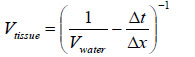 |
(25) |
where Vwater is the longitudinal wave velocity in water, Δt is time of flight from the 1st to the 2nd interface, and Δx is the thickness of the tissue.
Note that the tissue is compressed during the experiment. Therefore, it is difficult to measure the real thickness of the tissue precisely. Further, without the cover, no signal from the surface of the tissue can be seen. The longitudinal wave velocity of the tissue can be more accurately obtained with V(z) analysis [76-78].
4.7. Frequency Analysis
When an acoustic wave travels in a specimen, its amplitude decreases with the distance it travels. Eventually, it decays completely. There are a few useful methods to detect the attenuation in a skin tissue using the SAM (pulse-wave mode). The simplest way is to analyze the signal loss in the frequency domain using FFT analysis. This method is effective when the surface roughness of the specimen is not significant as compared with the wavelength of the transducer. We briefly describe the procedures of this method below.
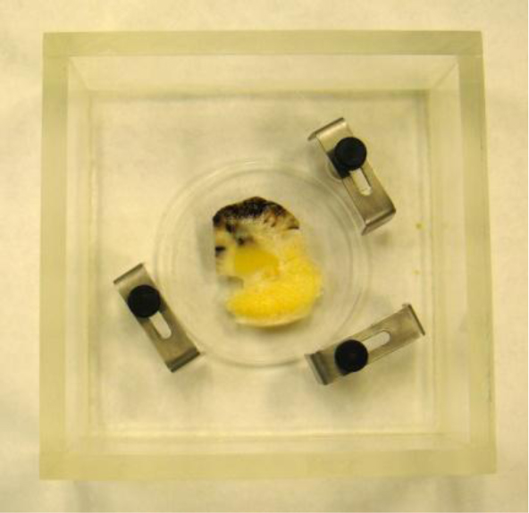
In this case, we need to locate the specimen on the substrate without the cover. As can be seen in Fig. (20), the thick melanoma tissue is located on the sapphire substrate (thickness: 1.78 mm), and there is no transparent poly-silicon cover on the front surface of the specimen.
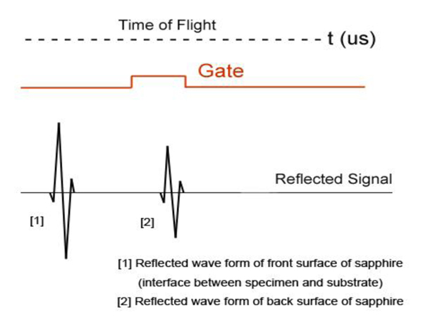
The schematic diagram of the experimental setup is shown in Fig. (21a).
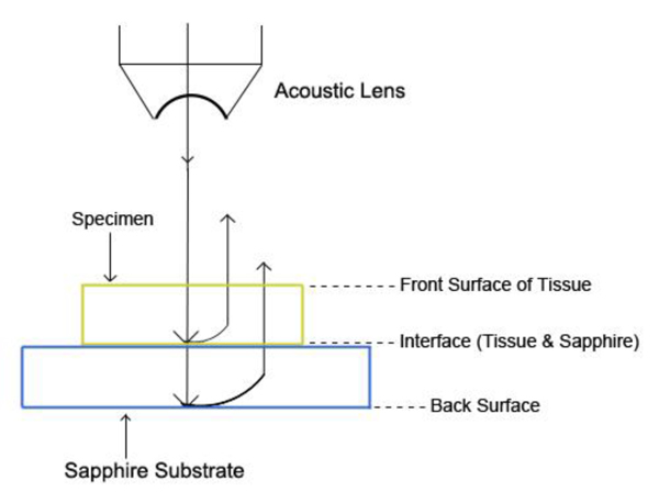
The diagram shows acoustic beams reflected from the specimen when attenuation is measured. In this setup, a specimen is placed on a sapphire substrate without a transparent poly-silicone cover. No acoustic wave reflected from the front surface of the specimen is seen on the monitor of the oscilloscope because the acoustic impedances of the water and the specimen are similar. In this case, the acoustic wave is primarily focused on the surface of the substrate. Therefore, the image is comprised of the information from the front surface of the specimen relative to the back surface of the specimen.
Fig. (21b) illustrates conceptual waveforms of the longitudinal wave reflected from the interface between the tissue and the front surface of the sapphire substrate, and that reflected from the back surface of the sapphire substrate (Fig. 21a). In reality, due to the high attenuation property in thick biological tissue specimens, the reflected wave from the back surface of the sapphire is hardly detectable. The signal loss calculated in this case is caused by the attenuation in the specimen only. To evaluate the correct signal loss in the tissue, the attenuation in water must be measured.
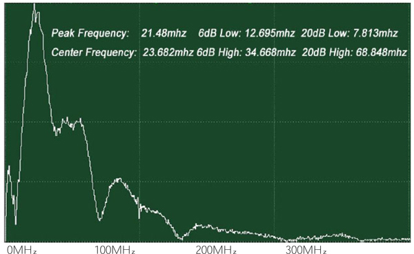
The attenuation can be evaluated simply from the FFT of the reference signal (Fig. 22). In this case, the acoustic lens emits an acoustic beam having a center frequency of 50 MHz. However, the frequency of the acoustic beam returned from the substrate in absence of tissue and any other scattering medium is 23.682 MHz. This indicates that the acoustic power corresponding to the difference in the center frequency of 50 MHz and 23.682 MHz is lost in water and other part in the path between the acoustic detector and the substrate. To evaluate the net signal loss in the specimen, this background loss must be subtracted from the apparent loss observed in the reduction of the center frequency.
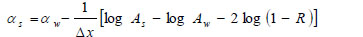
Alternatively, the acoustic attenuation coefficients of the specimen (denoted simply as “αs”) can be obtained from measured amplitude of reflected acoustic signal and calculation based on the following equation:
 |
(26) |
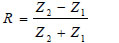
Here α is the attenuation coefficient, A is the amplitude of the received ultrasound pulse wave where indices S and W denote the specimen and water, Δx is the thickness of the specimen, and R is the acoustical reflection coefficient evaluated by the following equation [27]:
 |
(27) |
Here Zi= 1,2 are impedances of water and the specimen, respectively defined as
 |
(28) |
where ρi is the density and ci is the longitudinal wave velocity [79].
4.8. Shear Polarized Acoustic Lens
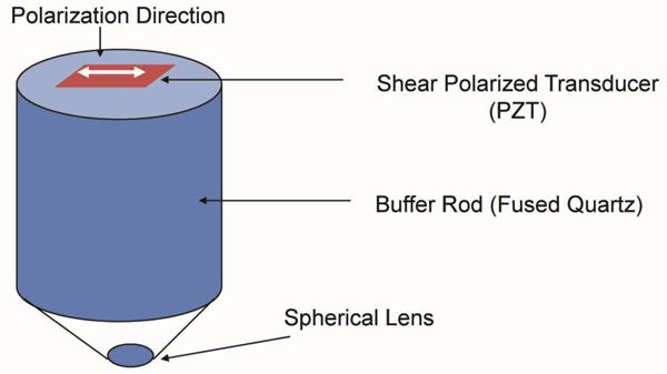
For anisotropic cancer such as a type of breast cancer, the shear polarized acoustic lens is useful. The acoustic beam excited in water with a shear wave transducer [80] has a directionality that allows visualization and/or measurement of anisotropy. Another advantage of using the shear wave transducer-lens system is that the signal transmitted into the water is directional along one axis, and there is no specular reflection from normal incidence on the specimen. Fig. (23) is a schematic diagram of a shear polarized acoustic lens. The acoustic lens comprises a buffer rod made of fused quartz, a shear polarized Piezoelectric Transducer (PZT) deposited in the rod. The opposite end of the rod has a spherical recess. Application of a voltage across the transducer excites a shear-polarized wave in the rod as shown by an arrow in Fig. (23). The wave travels downward to the lens. Mode conversion at the interface between the lens and the coupling medium excites the longitudinal wave. The wave is focused into the specimen via the coupling medium. The pattern of excitation of the longitudinal wave in the coupling medium is directional. Therefore, the anisotropy of a specimen can be visualized. The center frequency of the acoustic lens is 75 MHz.
4.9. Visualization of Anisotropy
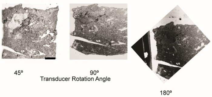
Fig. (24) shows images of the same breast cancer tissue formed by the above shear polarization acoustic lens. The specimen was rotated with three different angles (i.e., 45º, 90º, and 180º). The contrast of the image was changed in accordance with the direction of anisotropy. The left image clearly shows the group of the cancer cells. Applying this method to form a C-scan image of the breast cancer tissue, we do not need to deal with the gate width and the gate position. Further, we do not need to consider the decrease in the frequency of the pulse wave due to attenuation.
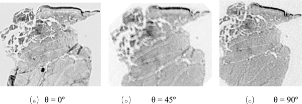
We used a shear polarized transducer-lens system (Fig. 23) to determine whether or not a thinly sectioned melanoma skin tissue is isotropic [1, 7]. The tissue was visualized with the transducer-lens system with frequency at 75 MHz. The tissue was rotated with the angles of 0º, 45º and 90º (Fig. 25). In this specimen, anisotropy was not observed. Since virtually no contrast difference was observed in the acoustic images when formed at different angles, we concluded that there is no or weak anisotropy.
CONCLUSION
Application of acoustic microscopy to the diagnosis of cancerous tissues has been discussed. Acoustic microscopy probes the object by examining the propagation characteristics of an acoustic wave reflected from a certain depth of the object. For the examination, the amplitude, phase (phase velocity), or both of the returning signals can be used. In any case, the difference in these parameters, due to abnormal cells in the medium, is visualized as a contrast to the normal cells. This basic principle of detection brings about two advantages. First, it allows us to examine living cells. As the mechanism of contrast forming relies on the natural properties of the medium, there is no need to stain or fix the specimen beforehand. Second, as the returning acoustic signal contains the phase information of all the points along the beam path, it can detect an abnormality at any point between the planes of reflection and detection. Further, by changing the focal plane inside the specimen, it is possible to enhance the information from a certain depth of the specimen. These advantages differentiate acoustic microscopy from optical microscopy that involves the use of an irreversible process to prepare the specimen and therefore is difficult to apply to the living cells.
Along with these advantages, acoustic microscopy has technical challenges in enhancement of the spatial resolution. To raise the spatial resolution, it is essential to use short wavelength. In a given medium, the resolution increases inversely proportional to the frequency. However, the attenuation of an acoustic wave increases in proportion to the square of frequency. Therefore, the returning signal is sharply weakened as the acoustic frequency is increased. It is thus difficult to increase both the spatial resolution and thickness of the specimen. The other technical challenge in biomedical application of acoustic microscopy is caused by the fact that living cells are composed of mostly water. This means that the acoustic impedance is more or less the same at all points in the object, lowering the reflection. Even if the reflected beam is strong, the contrast at the detection plane is low because the cancerous cells and normal cells have similar propagation characteristics.
Generally speaking, the above-mentioned issues are unique to either acoustic microscopy or optical microscopy. From this viewpoint, the acoustic and optical methods compensate each other for the respective shortfalls. In many applications, the two methods can be combined for a more accurate diagnosis.
NOTES
1 Some experimental data used in this paper are obtained by Y. Tien under the supervision of C. Miyasaka.
CONSENT FOR PUBLICATION
Not applicable.
CONFLICT OF INTEREST
The authors declare no conflict of interest, financial or otherwise.
ACKNOWLEDGEMENTS
Declared none.