All published articles of this journal are available on ScienceDirect.

Spatially Extended fMRI Signal Response to Stimulus in Non-Functionally Relevant Regions of the Human Brain: Preliminary Results
Abstract
The blood-oxygenation level dependent (BOLD) haemodynamic response function (HDR) in functional magnetic resonance imaging (fMRI) is a delayed and indirect marker of brain activity. In this single case study a small BOLD response synchronised with the stimulus paradigm is found globally, i.e. in all areas outside those of expected activation in a single subject study. The nature of the global response has similar shape properties to the archetypal BOLD HDR, with an early positive signal and a late negative response typical of the negative overshoot. Fitting Poisson curves to these responses showed that voxels were potentially split into two sets: one with dominantly positive signal and the other predominantly negative. A description, quantification and mapping of the global BOLD response is provided along with a 2 × 2 classification table test to demonstrate existence with very high statistical confidence. Potential explanations of the global response are proposed in terms of 1) global HDR balancing; 2) resting state network modulation; and 3) biological systems synchronised with the stimulus cycle. Whilst these widespread and low-level patterns seem unlikely to provide additional information for determining activation in functional neuroimaging studies as conceived in the last 15 years, knowledge of their properties may assist more comprehensive accounts of brain connectivity in the future.
1. INTRODUCTION
Analysis of data sets in functional neuroimaging via magnetic resonance (fMRI) is based on the haemodynamic response function (HDR) and the phenomenon of blood-oxygenation level dependency (BOLD). In this paper we demonstrate that for one dataset, a spatially varying HDR model can be fit across the whole brain, leading to a coherent global spatial structure of positive and negative responses in the HDR parameters. We present the results from this dataset as interesting preliminary findings, providing evidence for the existence of a neurally driven blood redistribution mechanism.
Haemoglobin is paramagnetic (has positive magnetic susceptibility in an external magnetic field) when de-oxygenated, but is diamagnetic (has negative susceptibility) when oxygenated. Therefore, the magnetic susceptibility of blood is altered depending on the relative concentration of deoxy-haemoglobin [1]. Brain activity requires the local consumption (metabolisation) of oxygen, forcing an increase in the flow rate and volume of cerebral blood that is much greater than the rate at which oxygen is metabolised, thereby leading to an increase in venous blood oxygenation. An increase in concentration of oxy-haemoglobin causes an increase in BOLD signal (reduced attenuation due to de-oxyhaemoglobin) and the change in this concentration over time defines the BOLD HDR (Fig. 1).
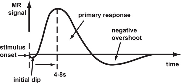
Schematic of the BOLD HDR morphology. Stimulus onset is shown by the first dashed line. The response takes the form of an initial dip (seen only at high magnetic field strengths) followed by a large positive response and then a negative overshoot which dips below the baseline.
In fMRI brain activation studies, the (BOLD) HDR is the core phenomenon being measured with the assumption that it represents underlying brain activity. The initial dip in oxygenation levels, detectable at high field strengths [2-5] is thought to be due to highly local micro-vascular depletion, though there is some debate as to whether it is robustly detectable with fMRI [6-8]. This is followed by the large over-compensation in oxygenated blood delivery to the site of activation detectable at lower field strengths. The HDR then falls a little more slowly than during the rise and subsequently dips below the baseline for a while (negative overshoot) before gradually returning to baseline. The source of the negative overshoot is not fully understood, but physiological mechanisms that have been proposed [9] include: 1) increased oxygen extraction rate due to sustained post-stimulus elevation in de-oxyhaemoglobin; 2) cerebral blood flow overshoot after stimulus ends; or 3) delayed recovery of venous cerebral blood volume.
Negative BOLD signals not attributable to the initial dip or negative overshoot have been observed in numerous activation studies [10, 11], and understanding the properties of such negative signals has been the object of considerable research [12-14]. Furthermore, the physiological interpretation of these negative BOLD signals is a debated topic, and suggested mechanisms include: 1) local vascular compensation or blood stealing [12]; 2) local decrease in neural activity [13, 14]; or 3) neurally controlled constriction of vessels as described in the discussion of Smith et al. (2004) [13]. As noted therein, if such a neurally controlled phenomenon genuinely exists, then it might be described as blood sharing rather than blood stealing since it reflects a global redistribution of blood through neuronally constricted and dilated vessels (haemodynamic balancing). Considerable human and animal research provides evidence that key physiological ingredients for a system capable of performing haemodynamic balancing exist [15, 16], with a range of possible neuronal triggering mechanisms [17-19].
When a single global delay is used for fitting the HDR, the magnitudes at voxels are inefficiently estimated by use of delays either too short or long, depending upon the difference between the particular delay imposed and the voxel’s ‘true’ delay. We have shown [20] that within ‘conventionally activated’ areas (i.e. regions of significant stimulus-responding activation) that there is up to a 4 s difference in delay of the HDR between voxels. In addition we found that magnitude estimates across conventionally activated areas are highly correlated with delay estimates. However, there is a large potential gain in statistical sensitivity for detecting stimulus-responding regions when fitting variable delay models to voxels with small response magnitudes, i.e. voxels outside the conventionally activated areas. In regions with smaller response magnitudes, the time to reach the peak of the response is relatively short. The ensuing discrepancy between the assumed fixed delay model and the true delay leads to systematic under-estimation of magnitude (which is already small). Fig. (2) illustrates the problem by showing the fit of a 10 s delay Poisson curve (defined later in the methods) to a 5 s delay Poisson curve with time to repetition (TR) of 1 s; the fitted curve’s magnitude is only 45% of that for the true response.
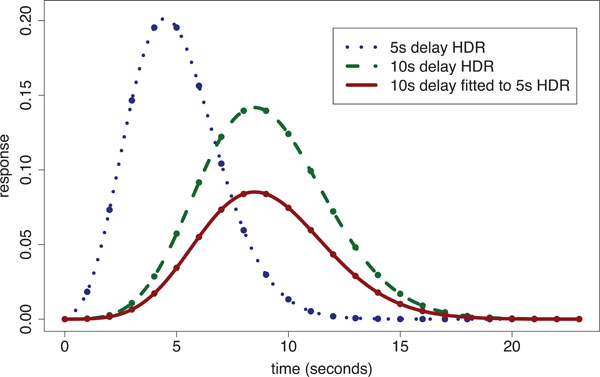
Poisson curve fitted HDR illustration: a 5 s delay Poisson generated ‘true response’ [dotted line shows Poisson points interpolated with a spline] is fitted using a 10s fixed-delay Poisson response template [dashed line shows spline interpolated 10 s delay Poisson curve with equal magnitude to that of the 5 s delay HDR] producing an underestimated fitted response [solid line]. The estimated magnitude is only 45% of the true response.
Given the underestimation from inappropriate delay assumptions, and the typically lower signal-to-noise ratios (SNRs) beyond these brain regions predicted to be activated by the stimulus, the signal from small magnitude voxels may not emerge from the noise to be detected as significantly active using conventional voxel-by-voxel thresholding-based tests, e.g. using Gaussian random fields [21]. (For conventionally restricted purposes of detecting direct stimulus-responding activation this may be a good thing.) Furthermore, the voxels that we show later to have a predominantly negative response (with delays of the order of that for the negative overshoot) would be missed by HDR models focused on matching the earlier positive response; the negative overshoot can continue up to 25 s beyond the end of the stimulus period - see e.g. Buxton (2002) [22] p. 418.
Previous attempts to detect spatial variation of delay across voxels [11, 23-27] were unable to detect the global response described here, probably because either 1) the form of delay variation they were capable of detecting was restricted by convolution assumptions and the need to choose canonical basis functions; 2) they were not looking for the possibility of extended regions of negatively responding voxels; 3) they did not directly estimate baseline levels of signal that were uncontaminated by negative overshoots from the response of a previous stimulus; 4) the effects would not appear significant using voxel-by-voxel thresholding-based tests. It is therefore informative to attempt to directly fit and assess a variable delay HDR model across all voxels in the brain to determine whether additional (possibly smaller magnitude) patterns of response emerge in both predicted and unpredicted brain areas; and if such patterns do emerge, to examine the possible implications on the underlying biology as well as on inferences derived from conventional activation and brain connectivity studies.
2. MATERIALS AND METHODOLOGY
Experimental Procedure
FMRI data were acquired using a T2*-weighted pulse sequence on a in-house built 3T scanner at the University of Nottingham Magnetic Resonance Centre [28], using a simple periodic ‘on/off’ auditory paradigm of 32 cycles. Each cycle contained 7 s of speech, followed by 28 s of silence to allow the HDR to return to baseline. Image volumes were acquired at 584 time points with a TR of 2.33 s. The stimulus was presented over background scanner noise and therefore the signal also contained a response to scanner noise. Each volume contained 8 contiguous coronal slices, consisting of regular lattices of 256 × 256 voxels. Voxel dimensions were 3 × 3 × 8 mm, the 8 mm being the slice thickness. The 8 coronal slices were situated to cover the temporal lobes (containing the auditory processing centres).
A healthy volunteer 25 year old male volunteer was requested to attend to the speech, but no response was required. The short stimulation period was used to prevent the MR signal reaching saturation, whereas the long silence period allows the signal to return to baseline before beginning the next cycle. A further 2 minutes of imaging in the silent condition (i.e. only background scanner noise) were acquired both directly before and after the experimental cycles. These additional scans were used to obtain stable baseline estimates, where here baseline means response to background scanner noise. Because the scanner noise happens at the same time as the image acquisition, its effects should appear as a constant background level of signal plus noise over the course of the experiment (including the baseline measurement periods). Motion correction was applied to correct for linear shifts in x, y and z and rotations around these axes. The data were spatially smoothed within SPM99 software [29] using a Gaussian kernel to stabilise parameter estimation, but were not temporally smoothed. Three different levels of spatial smoothing were examined: 1) no smoothing, 2) 3 mm full width at half maximum (FWHM), and 3) 5.5 mm FWHM. The 5.5 mm smoothing kernel was found to provide the greatest stability of fit, whilst still retaining spatial structure in the fitted parameter maps. The stability of fit was reduced when 3 mm kernel or no smoothing was performed. The reduced stability led to subsets of voxels not converging (a larger subset for the “no smoothing” case). However, among the voxels that did converge for the 3 mm kernel smoothed and unsmoothed datasets, the observed pattern of parameter estimates was similar to that of the fits for the 5.5 mm kernel smoothed data. The 5.5 mm choice of smoothing kernel (approximating to twice the voxel size) is consistent with the smoothness recommended by the conventional modelling approach implemented in Statistical Parametric Mapping (SPM). The individual voxel time series were high-pass filtered in SPM and any remaining linear trends were subsequently removed using linear regression.
Parameter Estimation
We fitted a HDR model directly to the average response curve at each voxel. This method contrasts with the usual approach of fitting a version of the stimulus function convolved with a canonical HDR or set of HDR basis functions to the voxel time courses. Avoiding convolution is preferable here in order to avoid the imposed restrictions on the shape of the HDR [20]. The HDR was modelled by a reference function hs(τ), where τ was the time from the onset of activity and s was the voxel location index. The fitting procedure has four steps:
- Estimate the baseline signal at each voxel by least squares using the two minute resting condition occurring immediately before and after the listening experiment and subtract the baseline estimate from the voxel data.
- Average the data across cycles to produce a ‘mean response’ cycle for each voxel.
- Fit a curve hs(τ) to each voxel's mean response cycle using least squares estimation.
- Create summary maps for the parameter estimates of the fitted curves.
In Kornak et al. (2009) [20] we compared a range of reference functions (gamma, constrained gamma, polynomials, and double gamma) for this direct fitting procedure. Here we forewent the options therein and instead fitted a simpler Poisson curve using the optimisation function nlregb in Splus (http://www.insightful.com/products/splus/default.asp).
The Poisson curve is defined as:
where T is the number of timepoints in the stimulus cycle and λs is the mean of the underlying distributional form for the Poisson curve at voxel s , providing for a measure of delay (in terms of scan intervals) at each voxel.
The Poisson curve, as defined here, shifts the functional form of the standard Poisson probability distribution one unit to the right; the first timepoint's response value is set to zero and each subsequent timepoint τ corresponds to the value of the distributional form at τ - 1. This shifted function is then scaled by a constant ks defined to be the response magnitude at voxel s . An implicit assumption of this model is that at time 0 of each cycle there is no response due to the stimulus.
The Poisson curve imposes an inherent constraint that the mean and variance are equal; the Poisson distribution is defined by the single parameter λ that equals both the mean and variance. Consequently, the Poisson curve imposes a specific non-linear relationship between delay and width (when defined in terms of FWHM or SD), and is therefore not invariant to changes in scale of the time axis. However, we found that the Poisson curve adequately modelled the main rise and fall of the HDR, while providing reliable fits for the design and dataset considered here. Examples of Poisson curve fits (Fig. 3). Summary parameter estimates from the Poisson curve fits θs =(ks,λs) (magnitude and delay, respectively) of hs(τ) were used to represent the nature of activation in each voxel.
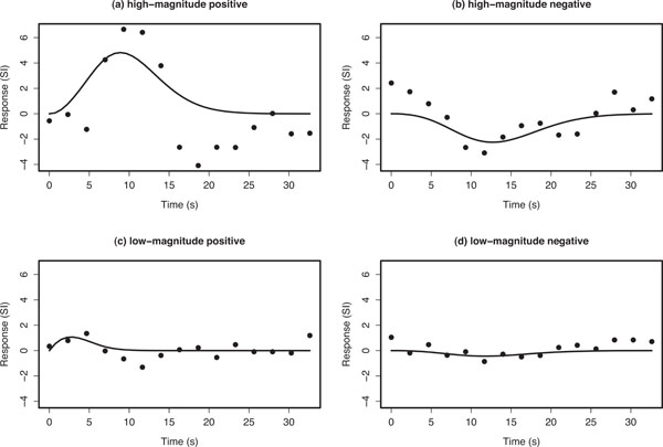
Example voxel timecourses for empirical average HDRs (points) and the corresponding Poisson curve fit (solid line). The fitted Poisson curve has been interpolated by a spline fit to provide a smooth fitted curve. Ordinate axes are in arbitrary units of signal intensity (SI) change.
It should be noted that non-stimulus locked activity and noise will be reduced relative to the signal in the empirically averaged cycles. Any systematic effects will be reduced because they are not synchronised to the stimulus and therefore do not behave additively when averaging, but rather tend to cancel each other out. The Poisson curve least squares fit implicitly assumes that noise exists in the average cycles, where the noise effectively includes all non-stimulus-locked forms of signal because non-stimulus-locked biological sources and signal noise cannot be separated. In addition, there will also be a component of signal due to the scanner noise that occurs every 2.33 s. However, since this signal will cycle at the frequency the data are acquired it should manifest as a constant additive effect. This constant additive effect should have been subtracted prior to the fitting of the Poisson because of the subtraction of the average of the two minutes of baseline at the beginning and end of the experiment.
The flexibility of allowing a spatially varying delay within a HDR model allows the Poisson curve to fit different types of responses. This flexibility of fit led to improved sensitivity for detecting spatial pattern in the magnitude and delay parameter maps, thereby enabling the findings reported here.
3. RESULTS
The baseline signal acquired in the 2 minute of ‘scanner noise only’ at the beginning and end of the experiments was very stable and proved important for obtaining stable estimates of haemodynamic response across all voxels. When comparing mean baseline estimates for the two minutes before and after experiments across all voxels, the mean absolute difference of ‘before’ and ‘after’ was 0.08 with a standard deviation of 0.06. This compares with an average absolute empirical signal change of 1.2 across all voxels (based on the maximal signal change of the 15 timepoints in the averaged cycles).
Fig. (4) shows parameter estimates for one coronal slice containing primary auditory cortex. For those voxels within core sites of the auditory cortex, a positive correlation between the Poisson curve magnitude parameter estimates (magnitude map) in panel (a) and the the corresponding map of estimates of delay (delay map) in panel (b) was seen over the first 10 s. These ‘conventionally active’ voxels can be seen in panel (a) as the set of high response magnitude voxels (dark region) on the left side of the map. However, beyond the principle regions of activity it was noticeable that the fitted magnitude parameters were spatially clustered into positive and negative magnitude voxels and that the delay map was inversely correlated with the pattern of the magnitude map; this pattern would be inconsistent with fitting to random noise. (The negative voxels, i.e., negative relative to baseline, would be detected as negative activation if found significant in a conventional fMRI analysis.) Since the Poisson curve fitting procedure from which the delay was obtained is identical for both positive and negative magnitudes, there was no asymmetry in the delay fitting procedure about zero magnitude, and therefore we would not expect the negative correlation in Fig. (4) between the magnitude (a) and delay (b) maps.
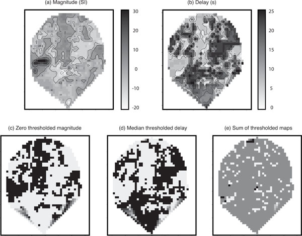
Parameter maps: (a) Poisson curve magnitude parameter estimates; (b) map of the corresponding delay parameters; (c) zero thresholded magnitude map. Black voxels correspond to positive magnitudes and white correspond to negative magnitudes; (d) the median thresholded delay map. Black voxels correspond to above median values and white voxels correspond to below medium values. Note the visible negative correlation with magnitude; and (e) the sum of the two thresholded maps. In the absence of a global effect this should contain roughly 25% black, 25% white, and 50% mid-grey. In all maps, darker regions correspond to higher values. Axes are on scales of mm. Note that when generating the images the software (Splus) provides extrapolation of the map to a convex hull around the observed set of voxels; hence the unusual triangular shape at the bottom of the slice.
Additional maps were generated from the original parameter estimates to illustrate this phenomenon more clearly. Panel (c) of (Fig. 4) displays a version of the magnitude map thresholded at zero with black voxels corresponding to positive magnitudes and white to negative. Panel (d) shows the delay map thresholded at its median value (black voxels consist of delays above the median), and panel (e) gives the sum of the two thresholded maps (c) and (d). The map in panel (e) of (Fig. 4) tends to homogeneous mid-grey (value =1). This is in contrast to what would be expected in the absence of a global haemodynamic effect. Under a null-hypothesis of no correlation between the length of the delay and whether a voxel is positive or negative responding you would expect to see an even split of positive and negative responding voxels above and below the median delay. Therefore, you would expect to see approximately 25% black ( = 2 ), 25% white ( =0 ) and 50% mid-grey (=1) in panel (e) of (Fig. 4). This result provides some insight into the reason for thresholding the delay at the median. If there is a 50-50 split of positive and negative responding voxels (which is approximately what we see), thresholding at the median of the delay is the optimal way to try and detect an association in a 2 × 2 table, i.e., we are looking for whether one 50-50 split can be assumed independent of another 50-50 split.
Fig. (3) shows typical empirical and fitted HDRs for the four main classes of voxel responses that we observed: high-magnitude positive- and negative-responding voxels, and low-magnitude positive- and negative-responding voxels. The first thing to note is that the empirical HDRs appear to exhibit both a positive and negative component. The Poisson curve is either completely above or below zero depending on the value of ks and is therefore only capable of fitting either the positive or negative component of the observed HDR.
The positive-responding voxels had a short delay compared with the negative ones. The fitted mean delays of positive responding voxels generally lay in a range matching the positive rise and fall of the HDR for conventionally responding voxels, whereas the fitted mean delays for the negative-responding voxels more closely matched typical delays for the negative overshoot; up to 28 s post stimulus e.g., Buxton (2002) [22] p. 418. Hence, over the time range of the delay estimates, there was a strong negative correlation between magnitude and delay. This contrasts with the smaller positive correlation seen when only the positive magnitude fits are considered. Two further observations are worthy of note. First, the observed pattern of effects occurred across the whole slice and was stimulus-locked, i.e. was temporally correlated with the stimulus paradigm. Second, the effect extended across brain regions that would not have been predicted a priori and in a conventional analysis would not have been detected as activity.
It is straightforward to confirm statistically that this global BOLD effect is not simply spatially correlated random variation. The test was performed based only on the voxels in the right half of the slice in Fig. (4) to avoid the left side that contained the peak activity. This region contained 643 voxels, whereas the whole slice contained 1236 voxels. If the null hypothesis were true, i.e. if the region only contained time courses formed from random noise (possibly temporally correlated) with zero mean, then the probability of obtaining a negative magnitude would be 0.5 for every voxel regardless of delay estimate.
Table 1 displays a 2 × 2 table of zero-thresholded magnitude against median-thresholded delay. A two-sided Fisher's exact test emphatically rejected the null hypothesis of no association between the sign of the magnitude and the size of the delay ( p<10-15 ). The cross-ratio measure of association for 2 × 2 contingency tables [30] was 499, implying a very high degree of association.
2 × 2 Contingency Table for Thresholded Parameter Estimates of the Displayed Slice: Magnitude Thresholded at Zero Versus Delay Thresholded at the Median Delay (3.372s)
| Magnitude < 0 | Magnitude > 0 | Row Totals | |
|---|---|---|---|
| Delay<median | 355 | 2 | 357 |
| Delay>median | 75 | 211 | 286 |
| Column totals | 430 | 213 | 643 |
Fig. (5) displays a scatter plot of delay against magnitude for all voxels, i.e., the complete set of slices covering the whole brain. The plot further indicates the strong asymmetry of the delay fits about the zero magnitude line. Those voxels designated as ‘conventionally activated’ comprised only a small proportion of voxels, and correspond to the dark region of high-magnitude positively responding voxels on the left side of (Fig. 4) (a). This set of voxel responses contrasts with the pattern expected if the remaining parameter estimates were based on white or temporally correlated noise, which would be approximately symmetric about the zero magnitude line. A further interesting feature of the plot is the group of low-magnitude negative responding voxels with a delay below 2 s. Spatially the largest group of these voxels lies to the bottom right of the main auditory area of activation -- see the light region below the main activated area in the delay map (b) of (Fig. 4). These voxels could potentially be interpreted as reflecting voxels with a dominant initial oxygenation dip. We defer comment on this to the discussion.
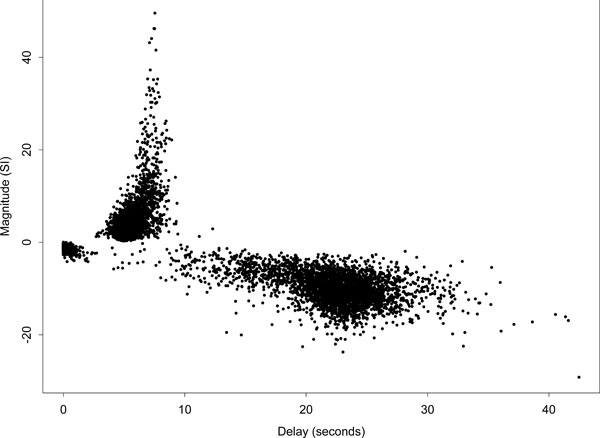
Scatter plot of delay against magnitude for the Poisson curve fits of all voxels in the brain. Ordinate axis is in arbitrary units of signal intensity (SI) change.
There are a few voxels with delays greater than 35 s because the Poisson curve fitted delay is not constrained to be less than 35 s. In addition, the fitted curve is only evaluated up to 35 s and therefore there is no signal beyond that to constrain the fitted curve to return quickly to zero. If the observed data across the cycle looks like it is a steady rise or decline it could be fit by a Poisson curve with a delay longer than the stimulus cycle.
Note that most of the voxels would not reach a level of conventional activation based on a “massively univariate” modelling approach, such as that used in SPM (i.e. voxel-by-voxel modelling followed by thresholding). The evidence that the voxels in this dataset do not consist of noise is primarily driven by the observation that most positive responding voxels have short delay and most negative ones have long delay (there is a consistent pattern across voxels that could not occur by chance). The highly significant Fisher's exact test result (which is still conclusive after conventionally activated voxels are removed) indicates that most of the brain is responding in a synchronised way to the stimulus. Because the Fisher's exact test as used here is essentially a global test of activation, we cannot say equivocally that any specific voxel is activated, but the very strong relationship in the 2 x 2 table indicates a very large proportion of voxels are “responding” in synchronicity with the stimulus.
Some alternative approaches within the Poisson curve fitting framework were examined, in order to relax the forced dichotomisation into all-positive or all-negative responses. First, the data were modelled using the sum of two Poisson curves, such that one was constrained to have a positive magnitude and the other a negative one. However, this formulation contained some non-identifiability, in that it was possible for the two curves to fully or partially cancel each other out. This led to the algorithm not converging in a high proportion of voxels, with the magnitude parameters tending to infinity for both the negative and positive directions. Even when the positive and negative delays were constrained to be within different ranges (according to expected positive delay and expected negative overshoot delay ranges), convergence problems persisted. The second approach was to force the fits for all voxels to be positive. Surprisingly, problems of non-convergence again occurred in many voxels, particularly those which had negative magnitudes in the original unrestricted fits. This suggests that although there appeared to be components of both positive and negative responses in most voxels, they could still be characterised in some sense as predominantly positive or negative responding.
4. DISCUSSION
Physiological Interpretation of Global Haemodynamic Effect
At this stage the physiological basis for the existence of a global haemodynamic effect (including ‘negative activation’), separate from conventional localised positive activation and residual noise, is not established. We briefly provide three possible alternate explanations for the observed global haemodynamic effect.
- At short distances from the activated area a complex haemodynamic balancing effect may be occurring, to compensate for the activation induced blood-flow in or near the neurally activated region. If the global effect comes from a haemodymaic balancing mechanism, we could expect some predominantly negative voxels nearby the conventionally activated area, but the explanation for the phase-locked activity throughout the brain remains more difficult. A global, stimulus invoked ‘ripple’ effect could be conceived with a neuronally driven balancing system; i.e., the blood sharing mechanism suggested in Smith et al. (2004) [13]. Such a neurally controlled vascular constriction and dilation mechanism would potentially lead to negative and positive BOLD signals that would not be a direct result of local neuronal activation. This mechanism would be consistent with the findings here, though considerable further investigation would be required to confirm this conjecture.
- The observed global response may be due to to the up- and down-regulation of a resting state default mode network. The suppression of a resting state network in the auditory system has been studied by Harrison et al. [31]. If the resting state network is suppressed when the subject is attending to the stimulus, then some of the signal that we we may be observing (delay > 7 s) could be due to the onset of the resting state mechanism post stimulus offset.
- High frequency respiratory/cardiac effects or other biological rhythms might have become synchronised with the experimental cycle. The high frequency effect signal could be observed within an average stimulus cycle as an aliased signal. However, these aliased high-frequency signals would probably not lead to Poisson fits with the spatial properties we observe over the brain (i.e. with correlation between sign of magnitude and delay).
If the global haemodynamic effect proves to be a physiological by-product (e.g. HDR balancing effect, resting state network regulation or chrono-synchronous physiological effects) and not an analysis artefact, it will be of interest for understanding brain function. Either way, when performing neuroimaging studies, this global effect provides a signal with spatial structure that can confound results. Therefore appropriately modelling this non-random pattern of response offers the possibility of improving the effective SNR for signals of interest in functional neuroimaging studies.
Possible Artefactual Explanations
We examined possible artefactual explanations for the global haemodynamic effect.
The first consideration was that the effect may be an artefact of the Poisson curve fitting procedure. However, if the fitting procedure was causing the effect in voxels that consisted of (possibly correlated) random noise (i.e. when there is no activation), then the Poisson curve would have similar properties whether fitting to positive or negative responding voxels. Specifically, there should be no correlation between the sign of the magnitude estimate and the delay, but this is in contradiction to the highly differential delays we see for positive versus negative responding voxels. It is possible that the choice of start values could influence the direction of fit, but we did not find that varying the start values affected the pattern of the fitted maps, only the probability of convergence.
The second possible artefactual cause considered was global re-scaling of the data performed in SPM99. Specifically, that the signal in the primary responding area may have caused a compensatory global re-scaling that spatially shifted signal to other areas of the brain (but in the opposite direction). However, if global re-scaling was the cause of the global haemodynamic effect, it would affect the signal by producing inverse HDRs in ‘non-active’ voxels. That is, the early positive signal would be subtracted, and the later negative overshoot added, to the voxel time courses. The global-scaling-adjusted voxel time courses across the brain would become negative for short delays and positive for long delays (in voxels originally consisting only of noise). This pattern is the opposite of what is observed and hence does not explain the global response.
The third possible artefact considered was that spatial smoothing may have induced the patterns of spatial correlation. Spatial smoothing could induce some spatial correlation in the signs of the fitted magnitudes. However, any induced correlation would necessarily be over relatively short distances for the Gaussian smoothing kernel of 5.5 mm FWHM. Therefore, the conventional activation in auditory cortex could not have induced the negative correlation structure between magnitude and delay in areas remote from the primary activation as displayed in Fig. (4).
Initial Dip Dominated Voxels
It is tempting to interpret the group of slightly negative responding voxels with a delay below 2 s in Fig. (5) as being caused by the initial dip in oxygenation level, observed in optical imaging and in fMRI at high field strengths, see Malonek and Grinvald (1996) [3]. However, when seen it was usually in voxels that then displayed a normal positive HDR and, since the first post-stimulus onset image is acquired 2.33 s after stimulation, it would be dangerous to assume that all voxels in this group were generated by a dominant initial dip. However, voxels with both a strong initial dip and a balance of later positive and negative phases (the combination of which did not obviously lean towards a fit in either direction) could lend themselves to fits reflecting the initial dip.
Temporally Correlated Noise and Nonlinear Estimation Limitations
When least squares fitting is used to estimate the Poisson curve parameters, no account is taken of temporally correlated noise [32]. However, it would be difficult to obtain reliable estimates of temporally correlated noise processes based on short averaged cycles since they would be confounded with the HDR response curve itself. The observed global response pattern could not be artefactually generated by a missed temporal correlation pattern because of the asymmetric delay values about zero magnitude.
Because the fitting of the Poisson curve is a nonlinear procedure it is conceivable that our parameter estimates find only a local mode of the least squares estimation function. This risk is reduced by our use of start values based on empirical magnitude estimates (sum of responses at each timepoint). The starting delay value was set at 4.66 s, i.e., corresponding to 2 TRs. The wide range of fitted delays (from 0 to over 30 s), the coherent relationship between the magnitude and delay parameters (see Fig. 5), and the convergence problems that occurred when restricting the fit to only positive magnitudes, together indicate that the procedure did not become trapped in an incorrect local minimum of the least squares estimation function. Furthermore, the results remained consistent despite changes in the starting delay parameter, except that some voxel estimates would not converge when the starting delay values were particularly low or high (close to 0 or above 5 TRs = 11.65 s).
5. CONCLUSION
The results in this paper for a single-subject dataset at high SNR show a global structure of HDR parameter estimates that is inconsistent with fitting to noise (even if the noise is temporally correlated). These results suggest the possibility of a haemodynamic balancing effect occurring outside of conventionally activated areas to compensate for highly localised oxygenated blood delivery. We are unable to determine any possible confounding effect which may produce these results artefactually, and assume that the effect becomes discernible through the extra flexibility obtained when employing a suitable spatially varying model for the HDR with adequate estimates of baseline BOLD signal. We acknowledge the limitation that the study is based on a single subject. It is a primary goal of this paper to encourage independent replication and further testing in terms of alternative sensory stimuli (visual, motor etc.) and different subject populations. If properties of this spatio-temporal effect are found to be generalisable, it raises far-reaching issues for techniques aiming to optimally localise activation and quantify brain connectivity in fMRI.
ACKNOWLEDGEMENT
This work was supported by 1) a UCSF Pilot Research Award to John Kornak; 2) the Medical Research Council United Kingdom as core programme of the Institute of Hearing Research and as postgraduate training studentship 5145 to John Kornak; and 3) NIH grants R01 AG032306 and P41 RR023953.