All published articles of this journal are available on ScienceDirect.

Measurements and Modeling of Transient Blood Flow Perturbations Induced by Brief Somatosensory Stimulation
Abstract
Proper interpretation of BOLD fMRI and other common functional imaging methods requires an understanding of neurovascular coupling. We used laser speckle-contrast optical imaging to measure blood-flow responses in rat somatosensory cortex elicited by brief (2 s) forepaw stimulation. Results show a large increase in local blood flow speed followed by an undershoot and possible late-time oscillations. The blood flow measurements were modeled using the impulse response of a simple linear network, a four-element windkessel. This model yielded excellent fits to the detailed time courses of activated regions. The four-element windkessel model thus provides a simple explanation and interpretation of the transient blood-flow response, both its initial peak and its late-time behavior.
1. INTRODUCTION
A detailed understanding of the neurovascular response in the brain is of critical value to science and medicine. Fundamentally, the neurovascular response is tightly linked in basic operation of the mind and brain. It seems likely that we will need a deeper understanding of vascular processes to grasp the strategies of neural computation. The success, in fact, of hemodynamic imaging techniques such as fMRI highlights the need for better understanding of neurovascular coupling. Specifically, knowledge of the vascular impulse response evoked by a brief (few seconds) stimulation would be useful. This is known as the hemodynamic response function (HRF). The HRF is formed by changes in oxygen uptake and blood flow. Measurements in cats [1, 2] and in rats, e.g., [3], indicate that the HRF typically exhibits a 3-phase response: an initial delay or dip lasting 2—3 s, a hyperoxic peak at 5—8 s, and an undershoot with frequent ringing. Because the brain is continually active, it is likely that such transient hemodynamic events occur continually throughout the brain. In order to understand the healthy operation of the brain, its pathophysiology, and the mechanisms of hemodynamic imaging, there is a need to better understand the hemodynamic processes that give rise to the HRF.
A number of models have been proposed for the dynamics of the HRF. The “balloon model” is the most popular [4, 5]. It explains the HRF based on flow and volume changes in the intra- and extravascular compartments with non-linear compliance. The volume changes were postulated to occur in venules and veins, as the global compliance of the venous system is known to be substantial [6-8]. A similar form for this model utilizes a lumped-element network analogy that includes a non-linear compliant element [9, 10]. Such models have become increasingly sophisticated and complex [11-13]. However, recent experiments have not shown much venular dilation; volume increases seem mostly to occur on the arterial side of the system [14, 15]. Accordingly, there is a need to revisit theoretical models for the HRF and its associated flow perturbation.
We propose a linear flow model, the four-element windkessel (FEW). This model, when combined with a convection-diffusion description of oxygen transport [16], provided excellent fits to oxygen measurements in tissue [1, 2]. In those results, the flow damping time constant suggested strongly underdamped responses. It is well known that the flow response of the HRF is mediated by the action of smooth-muscle fibers on the larger arterioles, and there is substantial evidence that pericytes modulate flow in small arterioles [17-20]. The flow response itself has been characterized extensively using such means as in vivo laser-Doppler flowmetry, e.g., [21-23], and laser speckle contrast imaging, e.g., [24-26]. Here we applied the FEW model to describe speckle-contrast measurements corresponding to flow-speed perturbations induced in rat somatosensory cortex by brief forepaw stimulation.
2. MATERIALS AND METHODOLOGY
Model
We model the flow perturbation using the FEW, a lumped linear equivalent-circuit model for the blood flow dynamics (Fig. 1A) [16]. The inertive element, I, models Newton’s 2nd law regarding the flow of blood in the pial arteries. The series resistance, R1 = R1a + R1b, represents frictional losses associated with the parallel combination of all downstream flow through the fractal vascular tree. The elements C and R2 represent the lossy compliance of the downstream venous vasculature. In steady state, and neglecting cardiac pulsatility, there is a constant pressure at point T, which represents the input to our model. The upstream vasculature, where flow perturbations are actively driven, couples resistively to the larger network, but the load resistance RA i s much greater than R1 and R2, so it does not perturb the global dynamics. The transient behavior of this system is modeled by the switch across R1b, which briefly closes to simulate a vasodilation that decreases the upstream vascular resistance. Because there was steady-state flow through I, the vasodilation creates a brief positive pressure fluctuation at T, which is described by the impulse response of the network.
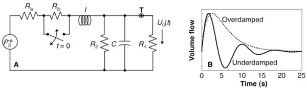
(A) FEW network; (B) impulse response
Because this system is linear, its impulse response fully characterizes its behavior. The flow perturbation impulse response has two forms depending upon the time constants of the system (Eqn.1).
The first form is under-damped and the second over-damped (Fig. 1B). The flow perturbation is specified by three parameters: the frequency f, khan damping time τ, and amplitude U10.
Animal Procedure
Three male Sprague-Dawley rats (250–350 g) were anesthetized with halothane (2%) and each animal was placed in a stereotaxic frame (Kopf Instruments, Tujunga, CA). A heating pad (WPI ATC1000) was used to maintain body temperatures of 37 °C. Then, in each rat, on the left hemisphere around the somatosensory cortex, a 4 mm × 4 mm portion of skull was thinned to transparency using a dental burr and then removed. A well was formed around the craniotomy using dental cement, which was then filled with silicone gel to improve visibility. Following surgery, animals were artificially ventilated with 1.5% halothane, 70% N2O and 30% O2, using procedures described previously [27].
All Animal Protocols were Approved by the Animal Care and Use Committees of the University of Texas at Austin.
Instrumentation
A laser diode (808 nm, 30 mW) and CMOS camera (Basler 602f, 610 × 490 pixels) were used to acquire laser speckle contrast imaging (LSCI) of blood flow in the cerebral cortex of each rat (Fig. 2) [25]. The laser diode was placed approximately 20 cm away from the animal at a 45° angle such that the area of interest was illuminated evenly. The scattered light was optically magnified between 1× and 3× depending on the animal. It was then captured by the camera at a rate of 100 frames/second and an exposure time of 5 ms. The acquisition was digitally recorded using custom software.
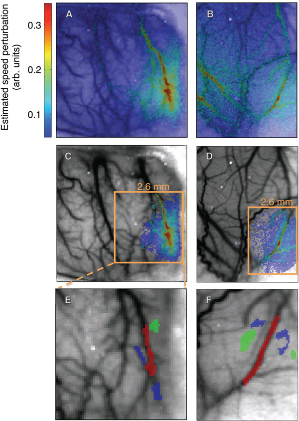
Measured flow perturbations in two animals: across the entire image (A, B), and restricted to a region where CNR ≥ 8 in animal 1 (C), and CNR ≥ 3.2 in animal 2 (D). Selected ROIs in this region (E,F): parenchyma, small blood vessels (blue), large blood vessels (red).
Experiment
The rat’s forepaw was electrically stimulated for 2 s starting 0.5 s after the trial onset. To induce somatosensory activity via electrical stimulation, needles were inserted between the digits, which were connected to a stimulus isolation unit (World Precision Instruments, Sarasota, FL). Current pulses of 1-2 mA were applied for 300 µs at a rate of 3 Hz for 2 seconds. The current level was adjusted to evoke a slight, visible twitch of one-or-more forepaw digits [27].
Forty trials with an inter-stimulus interval of 15 s were performed while image data were recorded at a rate of 100 frames/sec, which where then processed and displayed in real time [28]. The processed data were recorded for later analysis.
Speckle Contrast Image Analysis
The speckle contrast image is defined as the ratio of the standard deviation to the mean intensity in a small region of the image, K ≡ σs/<I>. The region must be chosen large enough that there is sufficient contrast to noise ratio, but not so large as to adversely limit our spatial resolution. With this in mind, a 7×7 region of pixels was empirically determined to balance these requirements; where each pixel is ~9 µm. A speckle contrast map was computed from the raw image using custom written softwareand downsampled to 10 frames/sec to improve signal-to-noise ratios (SNR) [25, 27].
Flow Computation
The speckle-contrast images were then converted to images of relative correlation times τc, , where K is the speckle contrast and T is the camera exposure time [29]. We used the temporal-mean of the correlation-time images as a structural image underlay for our results because of their apparent congruence with the vasculature (Figs. 2A, B). Larger blood vessels have higher blood speeds, yielding smaller correlation times, so the vasculature shows up as darker regions in the images.
To facilitate comparison with our flow model, we converted these values to a quantity related to blood speed. Since blood speeds may be assumed to be roughly inversely proportional to correlation times, we defined the normalized blood speed ν ≡ k / τc, where k is a proportionality constant [30]. We must be careful not to explicitly associate this with the local physical blood speed, as this assumption neglects numerous contributions to speckle contrast such as multiple scattering and penetration-depth effects [31]. To emphasize this loose connection, we denote the units of blood speed to be arbitrary. However, we chose k such that the average value of ν in regions of parenchyma equaled 0.7, the average blood speed in rat cerebral cortex parenchyma in mm/s. This provided a rough sense of the data in terms of real units [32]. Using this relationship, we created a spatial and temporal map of relative blood flow speed(454 × 433 pixels× 15 s × 40 trials). This was then spatially down sampled over a 4× 4 region to bring the dimensions to 113 × 108 pixels with pixel-size 36 µm.
To estimate the blood-flow response, we convolved the impulse response U1(t) (Fig. 1B) with a stimulus function, a 2-s-duration rectangular function (П) centered at t = 1.5 s:
F(t) = П[(t-1.5 s)/2]*[θ(t – 0.5 s)U1(t)]/20, where θ is a unit step function. This convolution served to approximate the vasodilation effects of the 2-s-duration somatosensory stimulus. The convolution stretched out the waveform causing an apparent ~0.5 s delay to the initial perturbation response. Although this flow perturbation is often strongly damped, with a 15-s ISI the perturbation may not decay to zero at the end of each trial. We included these effects by applying our model to a trial-averaged data set, where x and y refer to the coordinates of the pixel, t is time after trial onset, N is the total number of trials, and L is the trial length. Total blood speed is found by adding the baseline speed ν0 to the perturbation, ν(x,y) = ν0(x,y) + ν1(x,y,t).
We restricted our data analysis to pixels where activity exceeded a minimum contrast-to-noise ratio (CNR). The noise was estimated by computing the standard error about the mean for ν across trials and then averaged over the last third (5 s) of each trial. Contrast, which is the perturbation amplitude in this case, was estimated by taking the maximum blood speed in each pixel and subtracting the baseline blood speed (Fig. 2A). The baseline blood speed ν0 was computed by taking the mean of the normalized blood speeds in the last half-second of each trial. We then restricted our analysis to a contiguous region of pixels that exceeded a particular threshold (Figs. 2C, D). Within this region, we defined three compartmental regions-of-interest (ROIs) to illustrate response time series in large vessels, small vessels, and parenchyma (Figs. 2E, F).
To obtain fits we used MATLAB’s ls qcurvefit routine to perform non-linear optimization [33], varying the parameters U10, f, and τ to minimize the RMS error between the measurement and the model. We determined fit quality using the fraction of the variance explained, FOVE ≡ 1 – σ2fit – data / σ2data. We considered a fit to be successful if FOVE > 1 – 1/CNRmin, where CNRmin was the smallest CNR in the ROI (Fig. 2C-D)
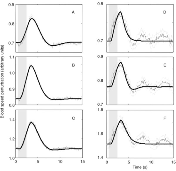
The experimental error per trial was defined to be the time averaged standard error of the mean over trials and is plotted as dotted lines in Fig. (3).
RESULTS
Good fits (FOVE > 80%) were obtained for all of the ROI time series data (Table 1 and Fig. 3). Mild ringing was observed in our fits to all of the sample ROIs in animals 1 and 3. All ROI fits in this animal were underdamped with significant undershoot. The fits observed in animal 3 were largely qualitatively similar to those observed in animal 1, and will not be further presented except to note a few relevant differences.
Fit Parameters for Vascular Compartment ROIs in the Three Animals
| Animal | ROI | FOVE (%) | f(Hz) | (s) |
|---|---|---|---|---|
| 1 | Parenchyma | 97.4 | 0.10 | 2.37 |
| Small Vessel | 99.4 | 0.090 | 1.62 | |
| Large Vessel | 99.2 | 0.094 | 1.74 | |
| 2 | Parenchyma | 82.4 | 0.0030 | 0.58 |
| Small Vessel | 85.4 | 0.17 | 1.26 | |
| Large Vessel | 83.0 | 0.0061 | 0.82 | |
| 3 | Parenchyma | 98.0 | 0.076 | 2.57 |
| Small Vessel | 97.9 | 0.080 | 2.51 | |
| Large Vessel | 97.6 | 0.070 | 2.32 |
Blood flow in animal 2 was distinctly different from the other two animals. FOVE was substantially smaller. The reduced fit quality was apparently caused by the presence of a ~0.2 Hz underdamped wave superimposed on a more typical strongly damped waveform. In addition, the hyperoxic peak exhibited a shorter duration. Fits for this animal showed less ringing, particularly for the large vessel and parenchymal compartments, but FOVE was smaller because the fits did not model the additional underdamped component.
We also fit our model to all of the pixel time series data that satisfied a minimum CNR threshold within the activated regions illustrated in Fig. 1. As noted previously, data from animal 2 had a much lower fit quality than the other two animals because of the apparently superimposed, stimulus-evoked ringing. The CNR threshold was therefore chosen to be less than in the other animals to produce an ROI that was similar in size to that of the other two animals. Mean parameter values for A, f and τ for those pixel time series that were successfully fit are summarized in Table 2. Fit frequency was similar in all animals. Damping time varied substantially, with the largest values (greatest ringing) in animal 3, while animal 2 exhibited the smallest values (greatest damping).
Fit Parameters, Median ± Standard Deviation, for the Activated Regions Illustrated in Fig. (1)
| Animal | CNRmin | Fit quality (%) | Amp. mod. (%) | A (arb. units) | f (Hz) | τ (s) |
|---|---|---|---|---|---|---|
| 1 | 8 | 88.7 | 21.0 ± 4.9 | 0.169 ± 0.054 | 0.090 ± 0.024 | 1.89 ± 0.42 |
| 2 | 3.2 | 29.0 | 14.0 ± 2.7 | 0.115 ± 0.036 | 0.107 ± 0.077 | 1.39 ± 0.90 |
| 3 | 12 | 99.3 | 26.9 ± 4.0 | 0.222 ± 0.052 | 0.077 ± 0.006 | 2.53 ± 0.24 |
| 1 | 8 | 88.7 | 21.0 ± 4.9 | 0.169 ± 0.054 | 0.090 ± 0.024 | 1.89 ± 0.42 |
| 2 | 3.2 | 29.0 | 14.0 ± 2.7 | 0.115 ± 0.036 | 0.107 ± 0.077 | 1.39 ± 0.90 |
| 3 | 12 | 99.3 | 26.9 ± 4.0 | 0.222 ± 0.052 | 0.077 ± 0.006 | 2.53 ± 0.24 |
There was a strong positive correlation between perturbation amplitude and baseline blood speed (R = 0.78, p < 10-16 in Fig. 4A and R = 0.77, p < 10-16 in Fig. 4C). Spatially, the perturbation amplitude appeared to largely follow the vasculature (Figs. 4B, D). The largest amplitudes were in one-or-two large blood vessels and then appeared to diminish toward their vascular periphery.
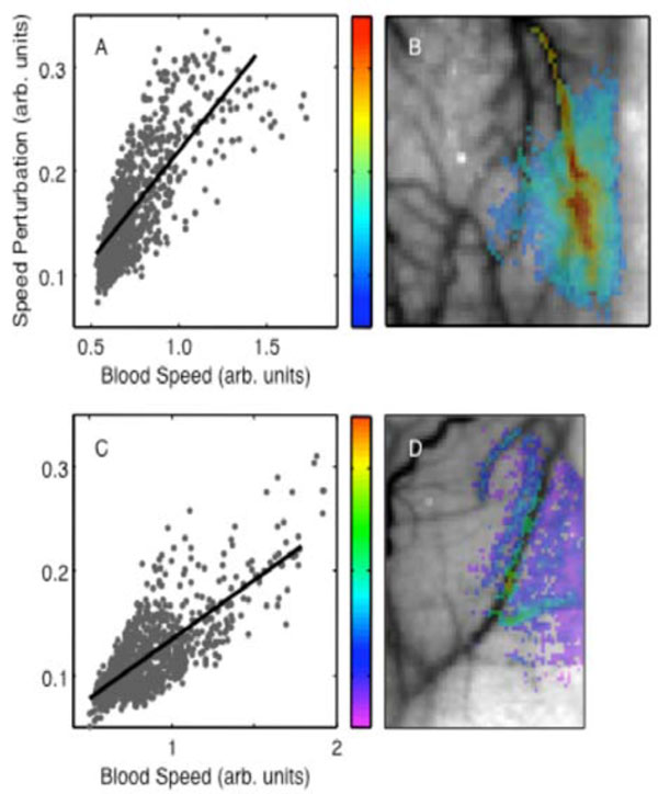
Perturbation amplitude parameter: (A) spatial distribution (animal 1); (B) dependence on baseline blood speed (animal 1). Animal 2: (C), (D).
In all animals, the frequency parameters exhibited a bimodal distribution (Figs. 5A, C). In animal 1, about 95% of the responsive pixels were better fit to an underdamped response with a mean frequency of 0.093 ± 0.016 Hz. About 5% were better fit to nearly critically damped responses; mean frequency in the lower mode is 0.0082 ± 0.0051 Hz. The mean frequencies in animal 2 were significantly higher in both the upper and the lower modes, 0.17 ± 0.02 Hz and 0.014 ± 0.008 Hz respectively. The strongly damped responses all corresponded to low baseline blood speed, suggesting that they occurred largely in parenchyma (ν0 < 1 ). There was a negative trend of frequency with flow speed for the high-frequency mode in animal 1 (R = -0.14, p< 0.02). Animal 2 showed a small positive trend in the upper mode (R = 0.24, p < 0.02). The frequency parameter showed a spatial distribution without a clear compartmental partition (Figs. 5B, D). In animal 1, the more strongly damped responses appeared mostly toward the right edge of the image, close to the edge of the craniotomy, while in animal 2 they were more central. The two modes seemed to occur largely in spatially distinct regions of the image.
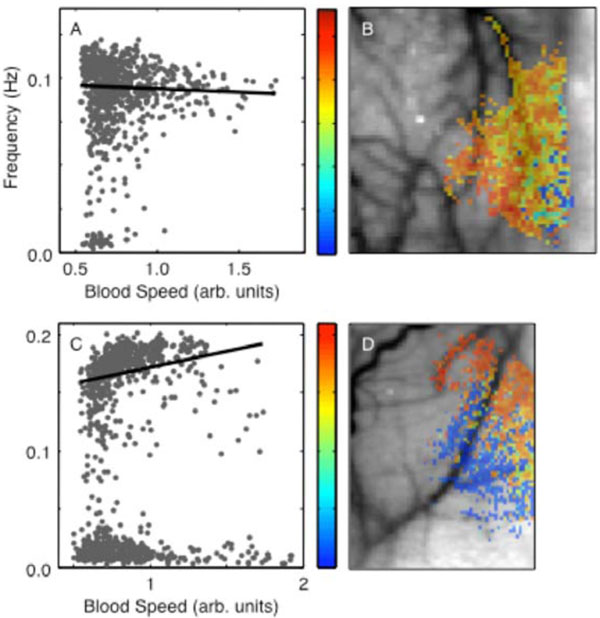
Perturbation frequency parameter: (A) spatial distribution in animal 1; (B) dependence on baseline blood speed, animal 1. (C) and (D) show correspondingdata in animal 2.
A weak but highly significant positive correlation was found between damping time and blood speed in both animals (R = 0.20, p < 6 × 10-11, Fig. 6B; R = 0.22, p < 1 × 10-13, Figs. 6A, C). Therefore, higher caliber vessels exhibited greater ringing. However, at lower blood speeds (parenchyma) we observed the widest range of damping time constants and some regions exhibited substantial undershoot (Fig. 3A). The damping time constant also showed a clear spatial trend, decreasing from upper left toward lower right in animal 1 (Fig. 6B) and from the upper right toward the lower left in animal 2 (Fig. 6D).
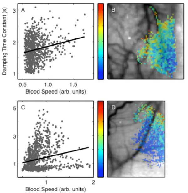
Perturbation damping time parameter: (A) spatial distribution in animal 1; (B) dependence on baseline blood speed in animal 1. (C) and (D) show corresponding data for animal 2.
3. DISCUSSION
Flow changes (blood speed) had a mean value of 20.6%, which is similar to other measurements, e.g., the ~30% flow changes obtained by positron emission tomography and MRI [34, 35]. The linear relationship between the perturbation amplitude and the baseline flow suggest that activation is, in fact, better revealed by a normalized flow metric. In animal 1, perturbation amplitude (Fig. 7A) suggests a region of activation toward the lower right that seems to follow the larger blood vessels. The normalized change in speed (Fig. 7B) illuminates a more spatially diffuse activation region. This confirms and partially explains the utility of fractional signal change as a standard metric in fMRI and functional optical imaging data analysis.
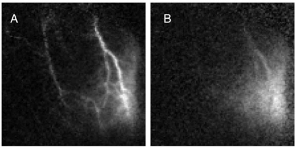
Perturbation amplitude (A) compared to relative fluctuation level (B).
We achieved good fits without modeling an initial period of latency or “initial dip” observed by other means. This suggests that the flow responses occurred promptly with stimulation and are not associated with transit-time delays from remote control points. The mean frequency parameter in the underdamped regime, ~0.08 Hz, was quite stable, suggesting that the pial vascular network behaves as a second-degree, roughly linear filter that is mechanically tuned to a particular frequency. Moreover, the median damping time of 1.9—2.5 s suggests that this network has a slightly underdamped, bandpass character.
The frequency fits were relatively stable with baseline flow speed, decreasing only slightly over a large range of baseline flow speeds and perturbation amplitudes. The stability of this parameter suggests that both the inertance and compliance parameters of the vasculature are also relatively stable. The stability of the compliance is very reasonable, because the compliance “seen” within the microvasculature will be strongly dominated by the downstream compliance of the venous tree, a global property. The inertance within the model corresponds to the mass of the blood regulated by the vascular control structures. Stability of the inertance would suggest that the key regulatory structures are spaced in a consistent stereotypical fashion in the cerebral microvasculature, perhaps at the level of the pial penetrating arterioles.
In contrast, the damping time showed a significant tendency to rise with blood speed. This is consistent with viscous flow properties in the smaller vessels where flow speeds are low, transitioning to laminar flow in the larger vessels where flow speeds are higher.
The spatial distribution of the flow responses showed an interesting bipartite distribution, with less damped responses occurring in one region, typically close to the focus of the activation, and more strongly damped responses occurring in more weakly activated regions. These observations suggest that the underdamped responses are more prevalent in microvascular regions closer to the regulatory source of the perturbation, and these responses become more damped in distal, venular portions of the microvasculature.
Our model did not as effectively fit the data observed in animal 2. This data appeared to exhibit a combination of a more strongly damped response, which was captured by our model, together with additional underdamped ringing at a higher frequency. This ringing is likely to be stimulus induced, because it is clearly evident and statistically significant after averaging over many trials. These data suggest the existence of more complex flow responses in response to repetitive transient stimulation. It is possible that such results could be modeled by more complex linear networks. For example, the measured flow response could be the superposition of flows mediated by two (or more) different mechanical regulation circuits, each with different time constants. Alternatively, the greater complexity could be introduced by neural feedback. On the other hand, these more complex responses could also be an artifact of the anesthesia, with little correspondence to the normal transient flow response.
Responses observed here were much more strongly damped than those observed in the tissue oxygen measurements obtained in cat visual cortex, ~2.2 s here versus ~9 s in cat [16]. The discrepancy could be explained in several ways. First, there could be delayed compliance effects that modify blood volume in a fashion distinct from flow changes. Delayed compliance has been a standard explanation used in many previous models [9-11, 13]. However, the absence of substantial volume changes in venular or capillary volume measurements [36] argues against this explanation because an increase in arterial blood volume alone cannot account for the large undershoots observed in both HbR and total Hb concentrations [3]. Another possibility is a species difference between rodents and cats. A third explanation concerns the level of anesthesia used in the experiments. In the cat experiments, anesthesia was maintained at a level light enough to permit significant neuronal activity as inferred by real-time EEG measurements. Such techniques were not used during the present experiments. The observed strongly damped responses, therefore, may have been caused by a different state of anesthesia. Our observation of more complex oscillatory responses in animal 3 suggests that neither the FEW model nor delayed compliance explanations may be sufficient to explain the HRF. Another possibility is that, for transient stimulation, visual cortex flow response is different, more underdamped, than that of somatosensory cortex. Further analysis and experiments will be necessary to establish the “normal” amount of ringing present in the flow response to brief neural activation.
The bandpass character of our flow model suggests an alternative explanation for some of the low-frequency oscillations or “vasomotion” observed with various techniques, e.g. [1, 32, 37-40]. Generally, these slow hemodynamic fluctuations have been attributed to mechanisms such as blood pressure feedback from baroreceptors or neurogenic mechanisms. These fluctuations, sometimes called Mayer waves, are observed in three frequency bands. The so-called “low-frequency” band of such fluctuations occurs at ~0.1 Hz, making it particularly relevant to the measurements and model presented here. The FEW has a bandpass response to transient changes in cerebrovascular control. Thus, unstimulated or spontaneous neural activity would be filtered by the hemodynamic network to appear as low-frequency oscillations in flow, oxygen transport, and other aspects of the hemodynamics. This hypothesis is consistent with the use of low-frequency fluctuations as a “resting-state” measurement of neural activity using fMRI [41-43]. The purpose of these oscillations is not yet understood. It has been suggested that low-frequency oscillations could increase oxygen transport efficacy [44, 45].
It could also be that several mechanisms are responsible for these fluctuations, with the FEW responsible only for fluctuations in hemodynamics associated with transient neural activation, while other neural feedback mechanisms, generally believed to be driven by blood CO2 concentrations (e.g., [46]), are responsible for oxygen auto-regulatory functions. It is also possible that the two mechanisms are related, with the tuned bandpass character of the cerebral vasculature being actually a consequence of the putative neurogenic feedback mechanisms. Although in global scope, the mechanism of the low frequency fluctuations may be complex and non-linear [47], at the level of the present cerebrovascular oxygen measurements they may be satisfactorily described by the FEW linear model. Although the FEW model is a substantial simplification of the complex flow dynamics associated with the whole of the cerebrovasculature, within the context of linear network models this kind of analogy has been utilized extensively to solve many problems. Complex networks of linear mechanical or fluid elements can always be converted to a Norton or Thevenin equivalent with a multi-pole admittance or impedance [48], and this approach has been utilized extensively in cardiovascular applications [8, 49, 50]. In this view, the dynamics of the FEW are an abstract model of more complex feedback mechanisms rather than a literal model of simple mechanical processes. Further experiments will be necessary to elucidate the relationship between the FEW and low frequency fluctuations.
ACKNOWLEDGEMENTS
We thank reviewer Junjie Liu for his many positive and helpful suggestions. Speckle measurement work was supported by the National Institutes of Health (EB008715, NS45879) and the American Heart Association (0735136N), and MERIT from the Department of Veterans Affairs.